
Loading...
Loading...
Loading...
Loading...
Loading...
Loading...
Loading...
Loading...
Loading...
Loading...
Loading...
Loading...
Loading...
Loading...
Loading...
Loading...
Loading...
Loading...
Loading...
Loading...
Loading...
Loading...
Loading...
Loading...
Loading...
Loading...
Loading...
Loading...
Loading...
Loading...
Loading...
A comprehensive guide to installing and licensing Motive.
Required PC specifications may vary depending on the size of the camera system. Generally, a system with more than 24 cameras will require the recommended specs to run properly.
OS: Windows 10, 11 (64-bit)
CPU: Intel i7 or better, running at 3 GHz or greater
RAM: 16GB of memory
GPU: GTX 1050 or better with the latest drivers and support for OpenGL 3.2+
USB C port to connect the Security Key
OS: Windows 10, 11 (64-bit)
CPU: Intel i7, 3 GHz
RAM: 4GB of memory
GPU that supports OpenGL 3.2+
USB C ports or an adapter for USB A to USB C to connect the Security Key
Download the Motive installer from the OptiTrack Support website. Click Downloads > Motive to find the latest version of Motive, or previous releases, if needed.
Both Motive: Body and Motive: Tracker use the same software installer.
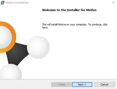
When the download is complete, run the installer to begin the installation.
When installing Motive for the first time, the installer will prompt you to install the OptiTrack USB Driver. This driver is required for all OptiTrack USB devices, including the Security Key. You may also be prompted to install other dependencies such as the C++ redistributable, which is included in the Motive installer. After all dependencies have been installed, Motive will resume its installation.
Follow the installation prompts and install Motive in your desired file directory. We recommend installing the software in the default directory, C:\Program File\OptiTrack\Motive.
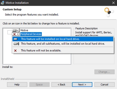
At the Custom Setup section of the installation process, you will be prompted to choose whether to install the Peripheral Devices along with Motive. If you plan to use force plate, NI-DAQ, or EMG devices along with the motion capture system, the Peripheral Devices must be installed.
If you are not going to use these devices, you may skip to the next step.
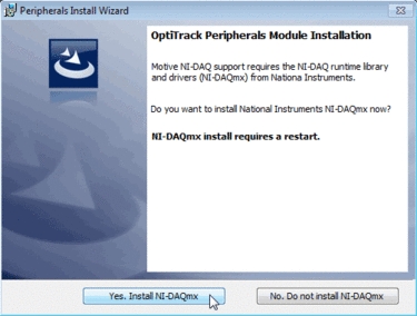
Peripheral Module NI-DAQ
After selecting to install the Peripheral Devices, you will be prompted to install the OptiTrack Peripherals Module along with the NI-DAQmx driver at the end of the Motive installation. Select Yes to install the plugins and the NI-DAQmx driver. This may take a few minutes to install and only needs to be done one time.
Once all the steps above are completed, Motive is installed. If you want to use additional plugins, visit the downloads page.
The following settings are sufficient for most mocap applications. The page Windows 11 Optimization for Realtime Applications has our recommended configuration for more demanding uses.
We recommend isolating the camera network and the host PC so that firewall and antivirus protection are not required. That will not be possible in situations where the host PC is connected to a corporate or institutional network. If so:
Make sure all antivirus software installed on the Host PC allows Motive traffic.
For Ethernet cameras, make sure the windows firewall is configured so the camera network is recognized.
Potential issues that can occur if antivirus software is installed:
Some programs (i.e., BitDefender, McAfee, etc.) may block Motive from downloading. The Motive software downloaded directly from OptiTrack.com/downloads is safe for use and will not harm your computer.
If you're unable to view cameras in the Devices pane, or you are seeing frame/data drops, verify that the antivirus or firewall settings allow all traffic from your camera network to Motive and vice versa.
Antivirus software may need to be completely uninstalled if it continues to interfere with camera communication.
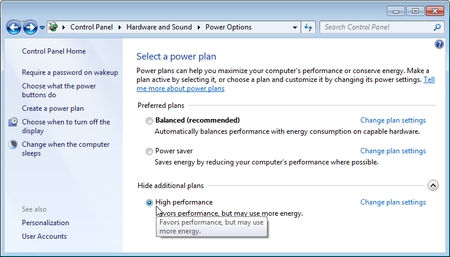
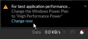
Windows power saving mode limits CPU usage, which can impact Motive performance.
To best utilize Motive, set the Power Plan to High Performance. Go to Control Panel → Hardware and Sound → Power Options as shown in the image below.
Required only for computers with integrated graphics.
Computers that have integrated graphics on the motherboard in addition to a dedicated graphics card may switch to the integrated graphics when the computer goes to sleep mode. This may cause the Viewport to become unresponsive when the PC exits sleep mode.
To prevent this, set Motive to use high performance graphics only.
Type Graphics in the Windows Search bar to find and open the Graphics settings, located at System > Display > Graphics.
In the Add an app field, select Desktop app, then browse to the Motive executable: C:\Program Files\OptiTrack\Motive\Motive.exe.
Motive will now appear in the list of customizable applications.
Click Motive to display, then click, the Options button.
Set the Graphics preference to High performance and click Save.
Once Motive is installed, the next step is to activate the software using the Motive 3.x license information provided at the time of purchase, and attach the USB Security Key. The Security Key attaches to the Host PC either through a USB C port or using an adapter for USB A to USB C.
Important Note about Licensing:
OptiTrack introduced a new licensing system with Motive 3. Please check the OptiTrack website for details on Motive licenses.
Security Key (Motive 3.x and above): Beginning with version 3.0, a USB Security Key is required to use Motive. The USB Hardware Keys that were used with older versions of Motive do not work with 3.x versions. To replace your Hardware Key with a Security Key, please contact our Technical Sales group.
Hardware Key (Motive 2.x or below): Motive 2.x versions require a USB Hardware Key.
Only one key should be connected at a time.
For Motive 3.0 and above, a USB Security Key is required to use the camera system. This key is different from the previous Hardware Key and it improves the security of the camera system.
Security Keys are purchased separately. For more information, please see the following page:
There are five types of Motive licenses:
Motive:Body-Unlimited
Motive:Body
Motive:Tracker
Motive:Edit-Unlimited
Motive:Edit
Each license unlocks different features in the software depending on the use case that the license is intended to facilitate.
The Motive:Body and Motive:Body-Unlimited licenses are intended for either small (up to 3) or large-scale Skeleton tracking applications.
The Motive:Tracker license is intended for real-time Rigid Body tracking applications.
The Motive:Edit and Motive:Edit Unlimited licenses are intended for users modifying data after it has been captured (post production work).
For more information on different Motive licenses, check the software comparison table on our website. An abbreviated version is available in the table below.
Quantum Solver
No
Yes
Yes
Yes
Yes
Live Rigid Bodies
Unlimited
Unlimited
Unlimited
No
No
Live Markersets & Skeletons
No
Up to 3
Unlimited
No
No
Edit Markersets & Skeletons
No
Up to 3
Unlimited
Up to 3
Unlimited
Track 6RB Skeletons
No
Yes
Yes
No
No
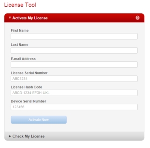
Motive licenses are activated using the License Activation tool. This tool can be found:
On the OptiTrack Support page.
On the Host PC at C:\Program Files\OptiTrack\Motive\LicenseTool.
On the Motive splash screen, when an active license is not installed.
Launch Motive. If the license has been activated, the splash screen will appear momentarily before Motive loads. If not, the splash screen will display the License not found error and a menu.
Click License Tool to open the License Activation Tool.
The License Serial Number and License Hash were provided on a printed card (enclosed in an envelope) when the license was purchased. If the card is missing, this information is also located on the order invoice.
The Security Key Serial Number is printed on the USB security key.
If you have already activated the license on another machine, make sure to enter the same name when activating it on the new PC.
Once you have entered all the information, click Activate. The license files will be copied into the license folder: C:\ProgramData\OptiTrack\License.
Click Retry to finish loading Motive.
Only one license (initial or maintenance) can be activated at a time. If you purchased one or more years of maintenance licensing, wait until the initial license expires before activating the first maintenance license. Let the first maintenance license expire before activating the next, and so on.
The Online License Activation tool allows you to activate licenses from the OptiTrack Support page. This option requires more steps but is helpful if you are activating licenses for multiple systems or do not have access to the host PC to use the license tool from the splash screen.
Enter the email address to send the license file(s) to in the E-mail Address field.
The License Serial Number and License Hash are located on the order invoice.
The Device Serial Number is printed on the USB security key.
If you have already activated the license on another machine, make sure to enter the same name when activating it on the new PC.
Once you have entered all the information, click Activate.
The license file(s) will arrive via email. Check your spam filter and junk mail if you don't see it in your inbox.
Download the license file(s) to the License Folder on the hard drive of the host PC: C:\ProgramData\OptiTrack\License.
Insert the USB security key, then launch Motive.
Notes on Connecting the Security Key
Connect the Security Key to a USB port where the USB bus does not have a lot of traffic. This is especially important if you have other peripheral devices that connect to the computer via USB ports. If there is too much other data flowing through the USB bus used by the Security Key, Motive might not be able to detect the key.
Make sure the USB Hardware Key for prior versions of Motive is not plugged in. If both the Hardware Key and the Security Key are connected to the same computer, Motive may not activate properly.
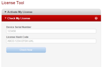
The Check My License tool allows you to lookup license information to obtain the expiration date.
About Motive Screen
About Motive includes information about the active license, which can be exported to a text file by clicking the Export... link at the bottom.
If Motive does not detect an active license, you can still open About Motive from the splash screen, however the only information available is the Machine ID.
You can install Motive on more than one computer with the same license and security key, but you will not be able to use it on multiple PCs simultaneously. Only the PC with the security key connected will be able to run Motive.
You can use the License Activation Tool to acquire the license files for the new host PC. This includes the initial license and any maintenance licenses that were purchased.
When run from the Motive splash screen, the tool will download the license files directly
When run from the OptiTrack Support website, the license files will be sent via emailed.
When using this method to transfer the license, enter the same contact information that was entered the first time the license was activated. We recommend exporting the license data to a text file from the original installation to use as a reference.
If the original information is lost, please contact OptiTrack Support for assistance.
The license file(s) can also be copied from one computer to another. License files are located at c:\ProgramData\OptiTrack\License. Open the license folder from the Motive Help menu.
If the files are copied from one PC to another, there is no need to re-run the License Activation Tool to begin using the currently active license. Simply install the version of Motive supported by the license and connect the security key.
For more information on licensing of Motive, refer to the Licensing FAQs from the OptiTrack website:
For common licensing issues and troubleshooting recommendations, please see the Licensing Troubleshooting page.
For more questions, contact OptiTrack Support:
Please attach the LicenseData.txt file exported from the About Motive panel as a reference.
Everything you need to know to move around the Motive interface.
This page provides an overview of Motive's tools, configurations, navigation controls, and instructions on managing capture files. Links to more detailed instructions are included.
In Motive, motion capture recordings are stored in the Take (.TAK) file format in folders known as session folders.
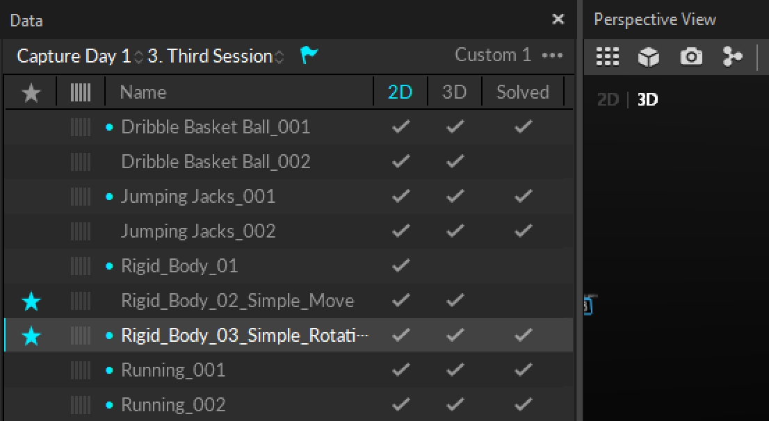
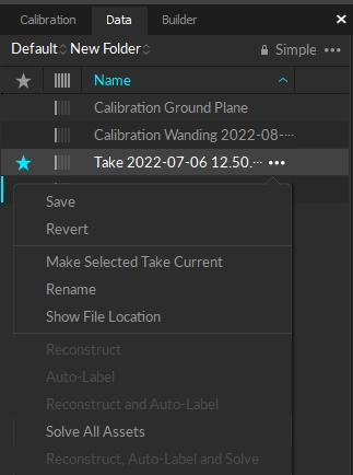
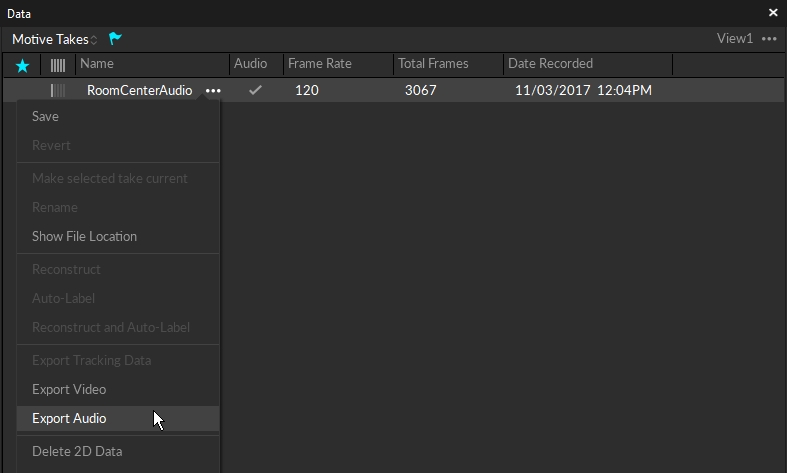
The Data pane is the primary interface for managing capture files. Open the Data pane by clicking the icon on the main Toolbar to see a list of session folders and the corresponding Take files that are recorded or loaded in Motive.
A .TAK file is a single motion capture recording (aka 'take' or 'trial'), which contains all the information necessary to recreate the entire capture, including camera calibration, camera 2D data, reconstructed and labeled 3D data, data edits, solved joint angle data, tracking models (Skeletons, Rigid Bodies, Trained Markersets), and any additional device data (audio, force plate, etc.). A Motive take (.TAK) file is a completely self-contained motion capture recording, that can be opened by another copy of Motive on another system.
Take files are forward compatible, but not backwards compatible, meaning you can play a take recorded in an older version of Motive in a newer version but not the other way around.
For example, if you try to play a take in Motive 2.x that was record in Motive 3.x, Motive will return an error. You can, however, record a Motive 2.x take and play it back in Motive 3.x.
If you have old recordings from Motive 1.7 or below, with .BAK file extensions, import them into Motive 2.0 and re-save them into the .TAK file format to open them in Motive versions 3.0 and above.
The folder where take files are stored is known as a session folder in Motive. Session folders allow you to plan shoots, organize multiple similar takes (e.g. Monday, Tuesday, Wednesday, or Static Trials, Walking Trials, Running Trials, etc.) and manage complex sets of data within Motive or Windows.
For a most efficient workflow, plan the mocap session before the capture and organize a list of captures (shots) to be completed. Type the take names in a spreadsheet or a text file, then copy and paste the list into the data pane. This will create empty takes (a shot list) with corresponding names from the pasted list.
Click the button on the toolbar at the bottom of the Data pane to hide or expand the list of open Session Folders.
Alternately, with the session folder list closed, click the name of the current session folder in the top left corner for a quick selection.
Please refer to the Session Folders section of the Data pane page for more information on working with these folders.
Software configuration settings are saved in the motive profile (*.motive) file, located by default at:
C:\ProgramData\OptiTrack\MotiveProfile.motive
The profile includes application-related settings, asset definitions, and the open session folders. The file is updated as needed during a Motive session and at exit, and loads again the next time Motive is launched.
The profile includes:
Application Settings
Live Pipeline Settings
Streaming Settings
Synchronization Settings
Export Settings
Rigid Body & Skeleton assets
Rigid Body & Skeleton settings
Labeling settings
Hotkey configuration
Profile files can be exported and imported, to maintain the same software configuration and asset definitions. This is helpful when the profile is specific to a project and the configuration and assets need to be used on different computers or saved for future use.
Please see the Export Assets Definition section of the Data Export page for more details.
To revert all settings to Motive factory defaults, select Reset Application Settings from the Edit menu.
A calibration file is a standalone file that contains all the required information to restore a calibrated camera volume, including the position and orientation of each camera, lens distortion parameters, and camera settings. After a camera system is calibrated, the .CAL file can be exported and imported back into Motive again when needed. For this reason, we recommend saving the camera calibration file after each round of calibration.
Reconstruction settings are also stored in the calibration file, in addition to the .MOTIVE profile. If the calibration file is imported after the profile file is loaded, the calibration may overwrite the previous reconstruction settings during import.
Note that an imported .CAL file is reliable only if the camera setup has remained unchanged since the calibration. Read more from the Calibration page.
The calibration file includes:
Reconstruction settings
Camera settings
Position and orientation of the cameras
Location of the global origin
Lens distortion of each camera
Default System Calibration
The default system calibration is saved at: C:\ProgramData\OptiTrack\Motive\System Calibration.cal
This file is loaded at startup to provide instant access to the 3D volume. The .CAL file is updated each time the calibration is modified or when closing out of Motive.
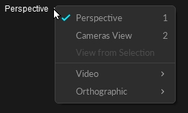
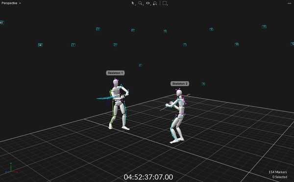
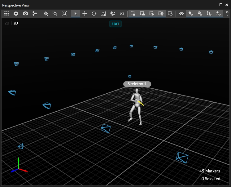
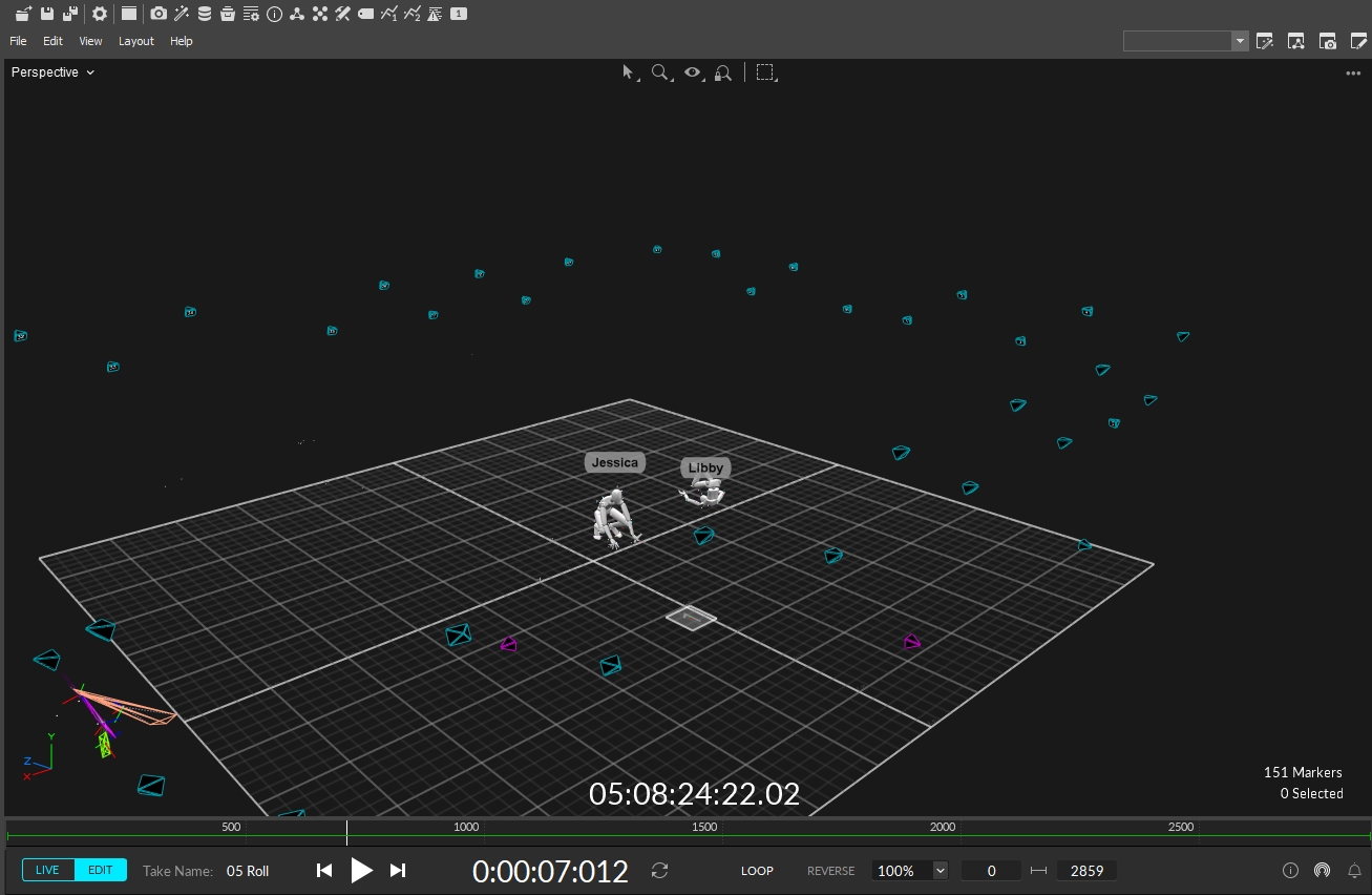
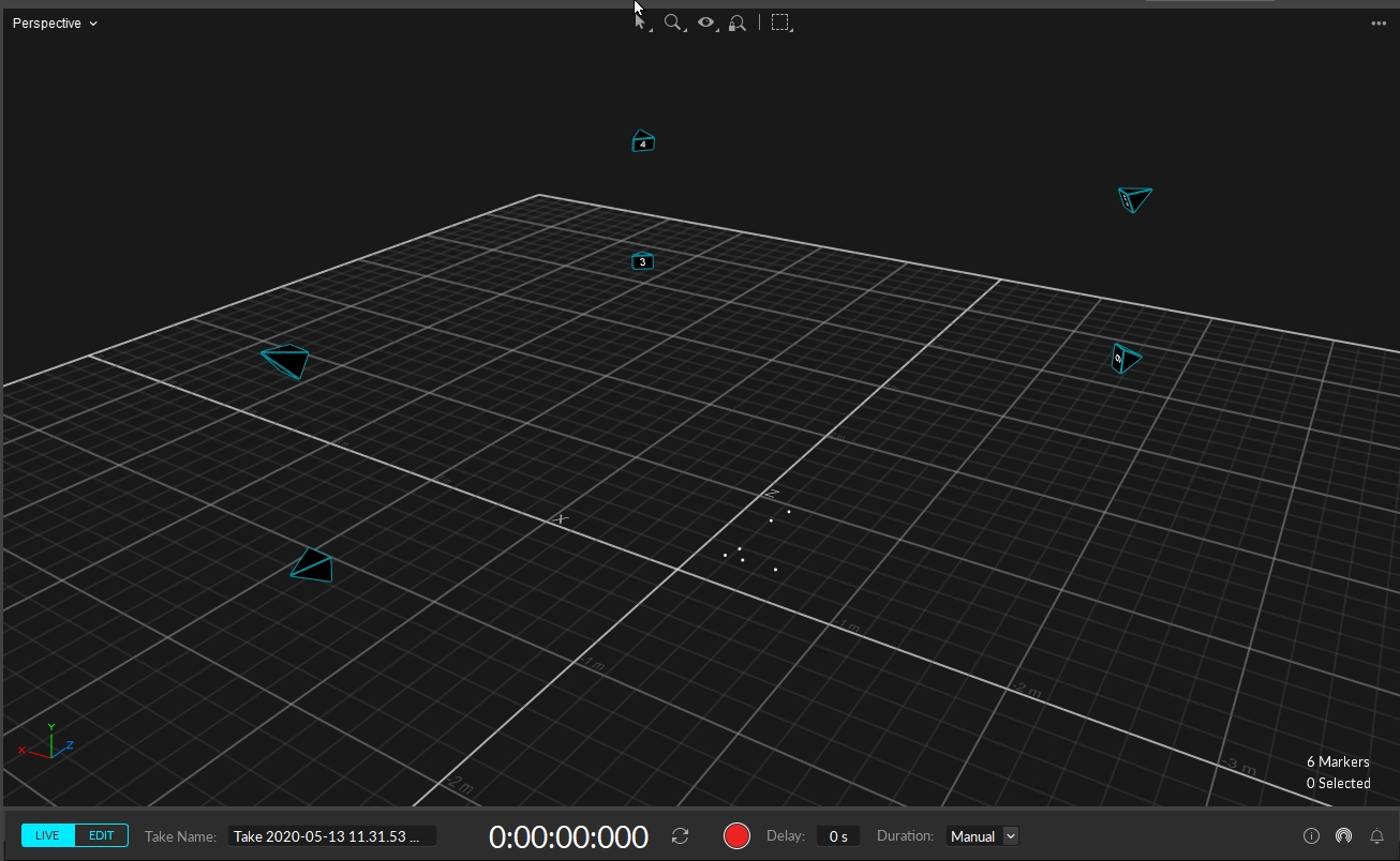
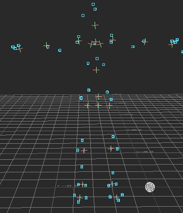
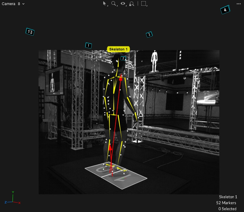
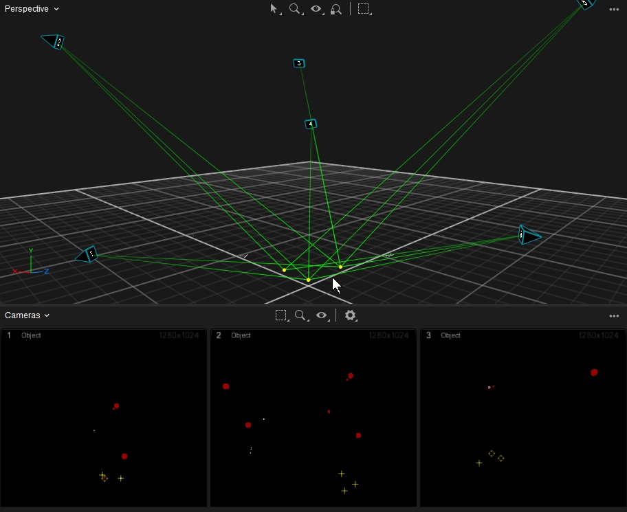
In Motive, the main viewport is fixed at the center of the UI and is used to monitor the 2D or 3D capture data in both live capture and playback of recorded data. The viewports can be set to either Perspective View, which shows the reconstructed 3D data within the calibrated 3D space, or Cameras View, which shows 2D images from each camera in the system. These views can be selected from the drop-down menu at the top-right corner. By default, the Perspective View opens in the top pane and the Cameras view opens in the bottom pane. Both views are essential for assessing and monitoring the tracking data.
Click on any viewport window and use the hotkey 1 to quickly switch to the Perspective view.
Displays the reconstructed 3D representation of the capture.
Used to analyze marker positions, view rays used in reconstruction, create assets, etc.
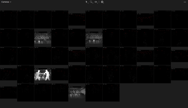
Click on any viewport window and use the hotkey 2 to quickly switch to the Cameras View.
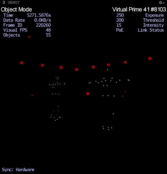
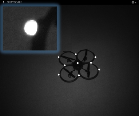
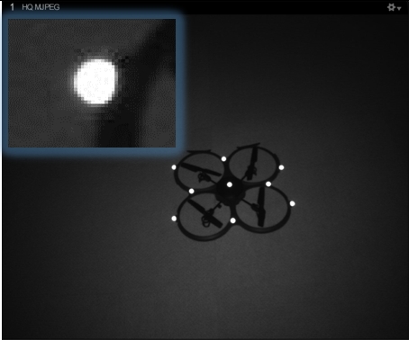
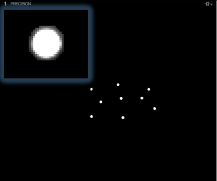
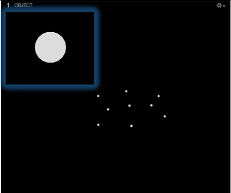
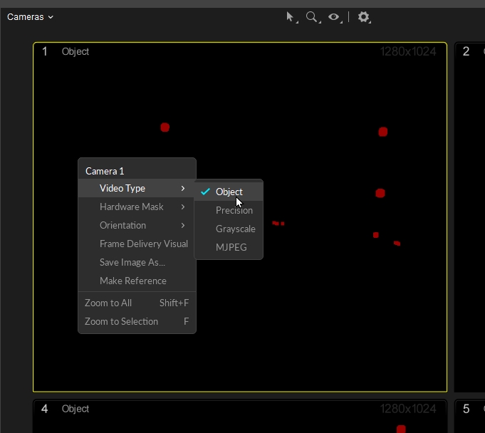
This view displays the images transmitted from each camera, with a header that shows the camera's Video Mode (Object, Precision, Grayscale, or MJPEG) and resolution.
Detected IR lights and reflections also show in this pane. Only IR lights that satisfy the object filters are identified as markers. See Cameras Basic Settings in the Settings: Live Pipeline page for more detail on object filters.
Includes tools to report camera information, inspect pixels, troubleshoot markers, and mask pixel regions to exclude them from processing. See Cameras View in the Viewport page for more details.
Most of the navigation controls in Motive are customizable, including mouse and Hotkey controls. The Hotkey Editor Pane and the Mouse Control Pane under the Edit tab allow you to customize mouse navigation and keyboard shortcuts to common operations.
The table below lists basic actions that are commonly used for navigating the viewports in Motive:
Rotate view
Right + Drag
Pan view
Middle (wheel) click + drag
Zoom in/out
Mouse Wheel
Select in View
Left mouse click
Toggle Selection in View
CTRL + left mouse click
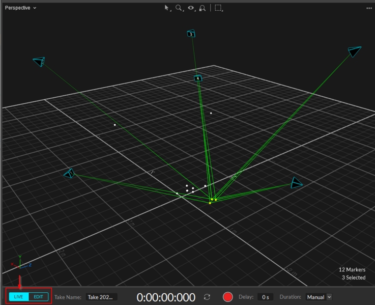
The Control Deck is always docked at the bottom of Motive, providing both recording and navigation controls over Motive's two operating modes: Live and Edit.
When using a timecode generator, you can control where the timecode data is displayed, either in the 3D view (default), in the Control Deck, or not shown at all.
From the Applications Settings panel, select Views -> 3D -> Heads Up Display -> Timecode.
All cameras are active and the system is processing camera data.
If the system is calibrated, Motive live-reconstructs 2D camera data into labeled and unlabeled 3D trajectories (markers) in real-time.
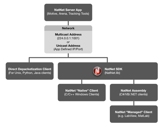
Live tracking data can stream to other applications using the data streaming tools or the NatNet SDK.
The system is ready for recording. Capture controls are available in the Control Deck.
Used for processing a loaded Take file (pre-recorded data). Cameras are not active.
Playback controls are available in the Control Deck, including a timeline (in green) at the top of the control deck for scrubbing through the recorded frames.
When needed, you can switch from editing in 3D to 2D mode, to view the real-time unreconstructed 3D data. Use this to perform a post-processing reconstruction pipeline to re-obtain a new set of 3D data.
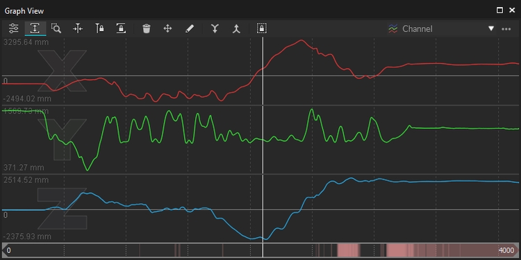
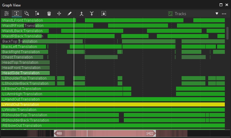
The Graph View pane is used to plot live or recorded channel data. There are many uses cases for plotting data in Motive; examples include tracking 3D coordinates of the reconstructed markers, 3D positions and orientations of Rigid Body assets, force plate data, analog data from data acquisition devices, and many more.
You can switch between existing layouts or create a custom layout for plotting specific channel data.
Basic navigation controls are highlighted below. For more information on graphing data in Motive, please read the Graph View pane page.
Hold the Alt key while left-clicking and dragging the mouse left or right over the graph to navigate through the recorded frames. You can use the mouse scroll also.
Scroll-click and drag to pan the view vertically and horizontally throughout plotted graphs. Dragging the cursor left and right pans the view along the horizontal axis for all of the graphs. When navigating vertically, scroll-click on a graph and drag up and down to also pan vertically.
Other Ways to Zoom:
Press Shift + F to zoom out to the entire frame range.
Zoom to a frame range by Alt + right-clicking the graph and selecting the specific frame range to zoom to.
When a frame range is selected in the timeline, press F to quickly zoom to it.
Frame range selection is used when making post-processing edits on specific ranges of the recorded frames. Select a specific range by left-clicking and dragging the mouse left and right, and the selected frame ranges will be highlighted in yellow. You can also select more than one frame ranges by holding the shift key while selecting multiple ranges.
The Navigation Bar at the bottom of the Graph View pane can also be used to
Left-click and drag on the navigation bar to scrub through the recorded frames. You can use the mouse scroll also.
Scroll-click and drag to pan the view range.
Zoom to a frame range by re-sizing the scope range using the navigation bar handles. As noted above, you can also do this by pressing Alt + right-clicking on the graph to select the range to zoom to.
The working range (also called the playback range) is both the view range and the playback range of a corresponding Take in Edit mode. In playback, only the working range will play, and in the Graph View pane, only the data for the working range will display.
Tip: Use the working range to limit exported tracking data to a specific range.
The working range can be set from different places:
In the navigation bar of the Graph View pane, drag the handles on the scrubber.
Use the navigation controls on the Graph View pane to zoom in or zoom out on the desired range.
The selection range is used to apply post-processing edits only to a specific frame range of a Take. The selected frame range is highlighted in yellow on both Graph View pane and the Control Deck Timeline.
When playing back a recorded capture, red marks on the navigation bar indicate areas with occlusions of labeled markers. Brighter colors indicate a greater number of markers with labeling gaps.
Motive's Application Settings panel holds application-wide settings, including:
Startup configuration and display options for both 2D and 3D viewports.
Settings for asset creation.
Live-pipeline parameters for the Solver and the 2D Filter settings for the cameras.
The Cameras tab includes the 2D filter settings that determine which reflections are classified as marker reflections on the camera views.
The Solver settings determine which 3D markers are reconstructed in the scene from the group of marker reflections from all the cameras.
To reset all application settings to Motive defaults, select Reset Application Settings from the Edit menu.
The Solver tab on the Live Pipeline settings panel configures the real-time solver engine. These are some of the most important settings in Motive as they determine how 3D coordinates are acquired from the captured 2D camera images and how they are used for tracking Rigid Bodies and Skeletons. Understanding these settings is very important for optimizing the system for the best tracking results.
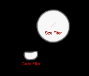
Under the Camera tab, you can configure the 2D Camera filter settings (circularity filter and size filter) as well as other display options for the cameras. The 2D Camera filter setting is a key setting for optimizing the capture.
For most applications, the default settings work well, but it is still helpful to understand these core settings for more efficient control over the camera system.
For more information, read through the Application Settings: Live Pipeline page and the Reconstruction and 2D Mode.
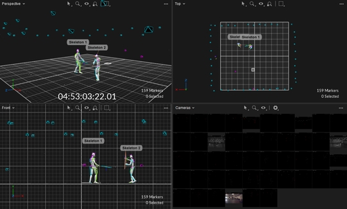
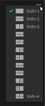
Motive includes several predefined layouts suited to various workflow activities. Access them from the Layout menu, or use the buttons in the top right corner of the screen.
The User Interface (UI) layout in Motive is highly customizable.
Select the desired panes from the View menu or from the standard toolbar.
All panes can be undocked to float, dock elsewhere, or stack with other panes with a simple drag-and-drop.
Reposition panes using on-screen docking guides:
Drag-and-drop the pane over the icon for the desired position. To have the pane float, drop it away from the docking guides.
Stacked panes form a tabbed window. The option to stack is only available when dragging a pane over another stackable pane.
Custom layouts can be saved and loaded again, allowing a user to easily switch between default and custom configurations suitable for different needs.
Select Create Layout... from the Layout menu to save your custom layout.
The custom layout will appear in the selection list to the left of the Layout buttons.
Custom layouts can also be accessed using HotKeys, with Ctrl+6 through Ctrl+9 set for user layouts by default.
Note: Layout configurations from Motive versions older than 2.0 cannot be loaded in latest versions of Motive. Please re-create and update the layouts for use.
Learn how to work with different types of trackable assets in Motive.
In Motive, an Asset is a set of markers that define a specific object to be tracked in the capture. Asset tracking data can be sent to other pipelines (e.g., animations and biomechanics) for extended applications.
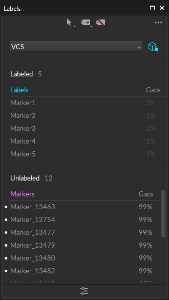
When an asset is created, Motive automatically applies a set of predefined labels to the reconstructed trajectories (markers) using Motive's tracking and labeling algorithms. Motive calculates the position and orientation of the asset using the labeled markers.
There are three types of assets, covering a full range of tracking needs:
Rigid Bodies: used to track rigid, unmalleable, objects.
Skeletons: used to track human motions.
Trained Markersets: used to track any object that is not a Rigid Body or a pre-defined Skeleton.
This article provides an introduction to working with existing assets. For information specific to each asset type, click the links in the list above. Visit the Builder pane page for detailed instructions to create and modify each asset type.
Assets can be created in Live mode (before capture) or in post-production (Edit mode, using a loaded TAKE).
If new assets are created during post-production, the take must be reconstructed and auto-labeled to apply the changes to the 3D data.
The following video demonstrates the asset creation workflow.
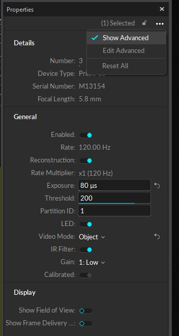
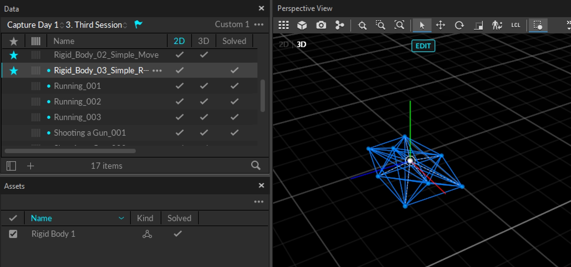
When an asset is selected, either from the Assets pane or from the 3D Perspective view, its related properties are displayed in the Properties pane.
Follow these steps to copy an asset to other recorded TAKES or to the Live capture.
Right-click the desired Take to open the context menu.
Select Copy Assets to Takes.
This will bring up a dialog window to select the assets to move.
Select the assets to copy and click Done.
Use shift-click or ctrl-click to select Takes from the Data pane until all the desired Takes are selected.
Right-click any of the selected Takes. This should copy the assets you selected to all the selected Takes in the Data pane to open the context menu.
Select Copy Assets to Takes.
This will bring up a dialog window to select the assets to move.
Select the assets to copy and click Done.
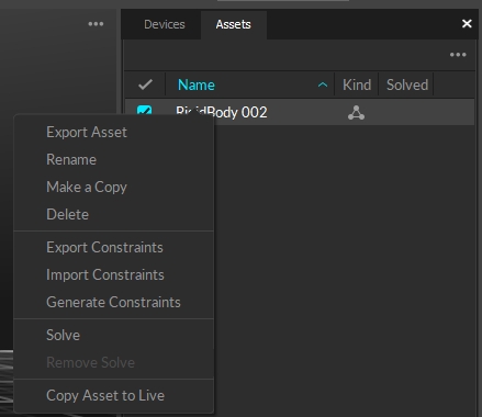
To copy multiple assets, use shift-click or ctrl-click to select all of them in the Assets pane.
Right-click (one of) the asset(s).
Select Copy Assets to Live.
The asset(s) will now appear in the Assets pane in Live mode. Motive will recognize the asset when it enters the volume, based on its unique marker placement.
Assets can be exported into the Motive user profile file (.MOTIVE), where they can then be imported into different takes without creating a new asset.
The user profile is a text-readable file that contains various configuration settings, including the asset definitions. With regard to assets, profiles specifically store the spatial relationship of each marker in the asset, ensuring that only the identical marker arrangement will be recognized and defined with the imported asset.
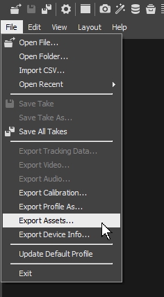
From the File menu, select Export Assets...
This will copy all the asset definitions in either Live-mode or in the current Take file into the user profile.
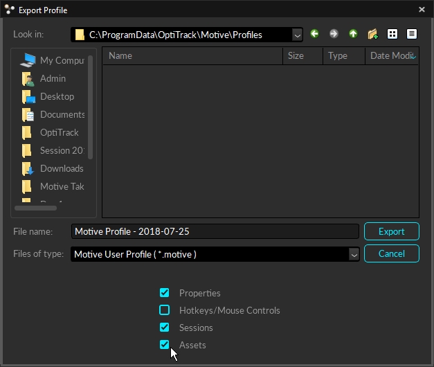
The option to export the user profile allows Motive users to save custom profiles as part of their project folders.
To export a user profile:
From the File menu, select Export Profile As...
The Export Profile window will open.
Navigate to the folder where you want the exported profile stored, or use the Motive default folder.
Select the profile elements to export. Options are: Properties, Hotkeys/Mouse Controls, Sessions, and Assets.
Name the file, using the File Type: Motive User Profile (*.motive).
Click Export.
OptiTrack motion capture systems can use both passive and active markers as indicators for 3D position and orientation. An appropriate marker setup is essential for both tracking the quality and reliability of captured data. All markers must be properly placed and must remain securely attached to surfaces throughout the capture. If any markers are taken off or moved, they will become unlabeled from the Marker Set and will stop contributing to the tracking of the attached object. In addition to marker placements, marker counts and specifications (sizes, circularity, and reflectivity) also influence the tracking quality. Passive (retroreflective) markers need to have well-maintained retroreflective surfaces in order to fully reflect the IR light back to the camera. Active (LED) markers must be properly configured and synchronized with the system.
OptiTrack cameras track any surfaces covered with retroreflective material, which is designed to reflect incoming light back to its source. IR light emitted from the camera is reflected by passive markers and detected by the camera’s sensor. Then, the captured reflections are used to calculate the 2D marker position, which is used by Motive to compute 3D position through reconstruction. Depending on which markers are used (size, shape, etc.) you may want to adjust the camera filter parameters from the Live Pipeline settings in Application Settings.
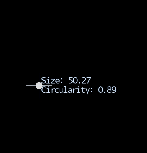
The size of markers affects visibility. Larger markers stand out in the camera view and can be tracked at longer distances, but they are less suitable for tracking fine movements or small objects. In contrast, smaller markers are beneficial for precise tracking (e.g. facial tracking and microvolume tracking), but have difficulty being tracked at long distances or in restricted settings and are more likely to be occluded during capture. Choose appropriate marker sizes to optimize the tracking for different applications.
If you wish to track non-spherical retroreflective surfaces, lower the Circularity value in 2D object filter in the application settings. This adjusts the circle filter threshold and non-circular reflections can also be considered as markers. However, keep in mind that this will lower the filtering threshold for extraneous reflections as well. If you wish to track non-spherical retroreflective surfaces, lower the Circularity value from the cameras tab in the application settings.
All markers need to have a well-maintained retroreflective surface. Every marker must satisfy the brightness Threshold defined from the camera properties to be recognized in Motive. Worn markers with damaged retroreflective surfaces will appear to a dimmer image in the camera view, and the tracking may be limited.
Pixel Inspector: You can analyze the brightness of pixels in each camera view by using the pixel inspector, which can be enabled from the Application Settings.
Please contact our Sales team to decide which markers will suit your needs.
OptiTrack cameras can track any surface covered with retro-reflective material. For best results, markers should be completely spherical with a smooth and clean surface. Hemispherical or flat markers (e.g. retro-reflective tape on a flat surface) can be tracked effectively from straight on, but when viewed from an angle, they will produce a less accurate centroid calculation. Hence, non-spherical markers will have a less trackable range of motion when compared to tracking fully spherical markers.
OptiTrack's active solution provides advanced tracking of IR LED markers to accomplish the best tracking results. This allows each marker to be labeled individually. Please refer to the Active Marker Tracking page for more information.
Active (LED) markers can also be tracked with OptiTrack cameras when properly configured. We recommend using OptiTrack’s Ultra Wide Angle 850nm LEDs for active LED tracking applications. If third-party LEDs are used, their illumination wavelength should be at 850nm for best results. Otherwise, light from the LED will be filtered by the band-pass filter.
If your application requires tracking LEDs outside of the 850nm wavelength, the OptiTrack camera should not be equipped with the 850nm band-pass filter, as it will cut off any illumination above or below the 850nm wavelength. An alternative solution is to use the 700nm short-pass filter (for passing illumination in the visible spectrum) and the 800nm long-pass filter (for passing illumination in the IR spectrum). If the camera is not equipped with the filter, the Filter Switcher add-on is available for purchase at our webstore. There are also other important considerations when incorporating active markers in Motive:
Place a spherical diffuser around each LED marker to increase the illumination angle. This will improve the tracking since bare LED bulbs have limited illumination angles due to their narrow beamwidth. Even with wide-angle LEDs, the lighting coverage of bare LED bulbs will be insufficient for the cameras to track the markers at an angle.
If an LED-based marker system will be strobed (to increase range, offset groups of LEDs, etc.), it is important to synchronize their strobes with the camera system. If you require a LED synchronization solution, please contact one of our Sales Engineers to learn more about OptiTrack’s RF-based LED synchronizer.
Many applications that require active LEDs for tracking (e.g. very large setups with long distances from a camera to a marker) will also require active LEDs during calibration to ensure sufficient overlap in-camera samples during the wanding process. We recommend using OptiTrack’s Wireless Active LED Calibration Wand for best results in these types of applications. Please contact one of our Sales Engineers to order this calibration accessory.
Proper marker placement is vital for quality of motion capture data because each marker on a tracked subject is used as indicators for both position and orientation. When an asset (a Rigid Body or Skeleton) is created in Motive, its unique spatial relationships of the markers are calibrated and recorded. Then, the recorded information is used to recognize the markers in the corresponding asset during the auto-labeling process. For best tracking results, when multiple subjects with a similar shape are involved in the capture, it is necessary to offset their marker placements to introduce the asymmetry and avoid the congruency.
Read more about marker placements from the Rigid Body Tracking page and the Skeleton Tracking page.
Asymmetry
Asymmetry is the key to avoiding the congruency for tracking multiple Marker Sets. When there are more than one similar marker arrangements in the volume, marker labels may be confused. Thus, it is beneficial to place segment makers — joint markers must always be placed on anatomical landmarks — in asymmetrical positions for similar Rigid Bodies and Skeletal segments. This provides a clear distinction between two similar arrangements. Furthermore, avoid placing markers in a symmetrical shape within the segment as well. For example, a perfect square marker arrangement will have ambiguous orientation and frequent mislabels may occur throughout the capture. Instead, follow the rule of thumb of placing the less critical markers in asymmetrical arrangements.
Prepare the markers and attach them on the subject, a Rigid Body or a person. Minimize extraneous reflections by covering shiny surfaces with non-reflective tapes. Then, securely attach the markers to the subject using enough adhesives suitable for the surface. There are various types of adhesives and marker bases available on our webstore for attaching the marker: Acrylic, Rubber, Skin adhesive, and Velcro. Multiple types of marker bases are also available: carbon fiber filled bases, Velcro bases, and snap-on plastic bases.
This page provides instructions on how to utilize the Gizmo tool for modifying asset definitions (Rigid Bodies and Skeletons) on the 3D Perspective View of Motive
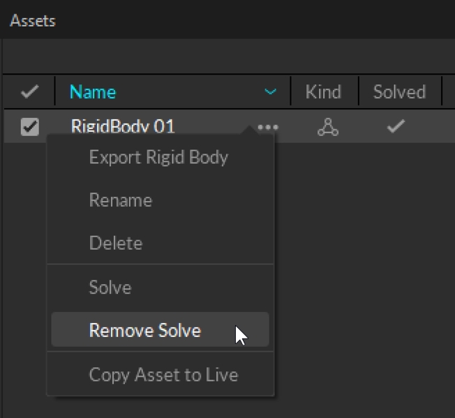
Edit Mode: As of Motive 3.0, asset editing can only be performed in Edit mode
Solved Data: In order to edit asset definitions from a recorded Take, corresponding Solved Data must be removed before making the edit, and then recalculated.
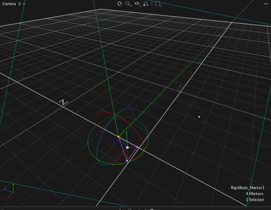
The gizmo tools allow users to make modifications on reconstructed 3D markers, Rigid Bodies, or Skeletons for both real-time and post-processing of tracking data. This page provides instructions on how to utilize the gizmo tools.
Using the gizmo tools from the perspective view options to easily modify the position and orientation of Rigid Body pivot points. You can translate and rotate Rigid Body pivot, assign pivot to a specific marker, and/or assign pivot to a mid-point among selected markers.
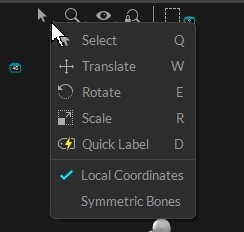
Select Tool (Hotkey: Q): Select tool for normal operations.
Translate Tool (Hotkey: W): Translate tool for moving the Rigid Body pivot point.
Rotate Tool (Hotkey: E): Rotate tool for reorienting the Rigid Body coordinate axis.
Scale Tool (Hotkey: R): Scale tool for resizing the Rigid Body pivot point.
Precise Position/Orientation: When translating or rotating the Rigid Body, you can CTRL + select a 3D reconstruction from the scene to precisely position the pivot point, or align a coordinate axis, directly on, or towards, the selected marker. Multiple reconstructions can also be selected, and their geometrical center (midpoint) will be used as the target reference.
Please note that the following tutorial videos were created in an older version of Motive. The workflow in 3.0 is slightly different and only requires you to select Translate, Rotate, or Scale from the 3D Viewport Toolbar selection dropdown to begin manipulating your Asset.
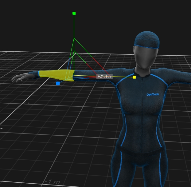
You can utilize the gizmo tools to modify skeleton bone lengths, joint orientations, or scale the spacing of the markers. Translating and rotating the skeleton assets will change how skeleton bone is positioned and oriented with respect to the tracked markers, and thus, any changes in the skeleton definition will affect the realistic representation of the human movement.
The scale tool modifies the size of selected skeleton segments.
The gizmo tools can also be used to edit positions of reconstructed markers.In order to do this, you must be working reconstructed 3D data in post-processing. In live-tracking or 2D mode doing live-reconstruction, marker positions are reconstructed frame-by-frame and it cannot be modified. The Edit Assets must be disabled to do this (Hotkey: T).
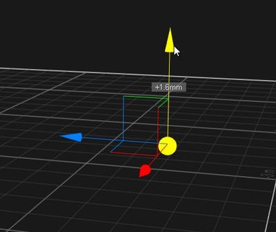
Translate
Using the translate tool, 3D positions of reconstructed markers can be modified. Simply click on the markers, turn on the translate tool (Hotkey: W), and move the markers.
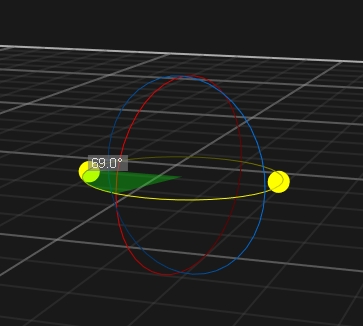
Rotate
Using the rotate tool, 3D positions of a group of markers can be rotated at its center. Simply select a group of markers, turn on the rotate tool (Hotkey: E), and rotate them.\
Scale
Using the scale tool, 3D spacing of a group of makers can be scaled. Simply select a group of markers, turn on the scale tool (Hotkey: R) and scale their spacing.
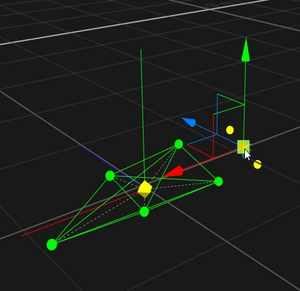
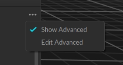
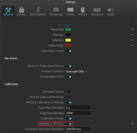
Cameras can be modified using the gizmo tool if the Settings Window > General > Calibration > "Editable in 3D View" property is enabled. Without this property turned on the gizmo tool will not activate when a camera is selected to avoid accidentally changing a calibration. The process for using the gizmo tool to fix a misaligned camera is as follows:
Select the camera you wish to fix, then view from that camera (Hotkey: 3).
Select either the Translate or Rotate gizmo tool (Hotkey: W or E).
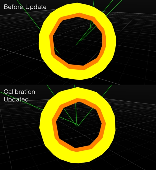
Use the red diamond visual to align the unlabeled rays roughly onto their associated markers.
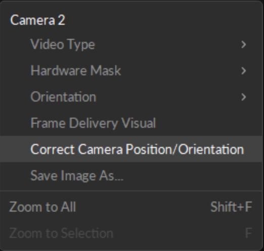
Right lock then choose "Correct Camera Position/Orientation". This will perform a calculation to place the camera more accurately.
Turn on Continuous Calibration if not already done. Continuous calibration should finish aligning the camera into the correct location.
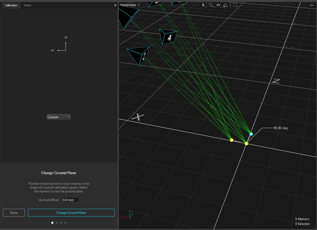
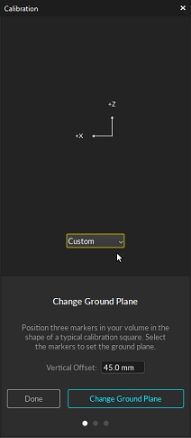
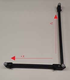
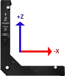
During process, a calibration square is used to define global coordinate axes as well as the ground plane for the capture volume. Each calibration square has different vertical offset value. When defining the ground plane, Motive will recognize the square and ask user whether to change the value to the matching offset.
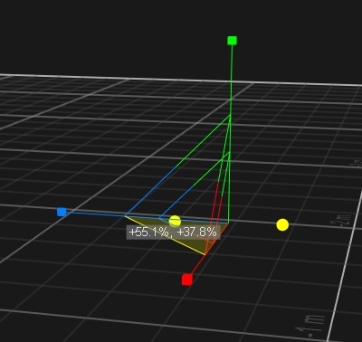
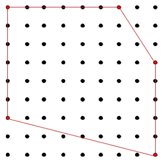
When creating a custom ground plane, you can use Motive to help you move the markers to create approximately 90 degree between the 3 markers. This is of course contingent on how good your calibration is, however, this will still give you a fairly accurate starting point when setting your ground plane.
Motive accounts for the vertical offset when using a standard OptiTrack calibration square, setting the origin at the bottom corner of the calibration square rather than the center of the marker.
When using a custom calibration square, measure the distance between the center of the marker and the lowest tip at the vertex of the calibration square. Enter this value in the Vertical Offset field in the Calibration pane.
The Vertical Offset property can also be used to place the ground plane at a specific elevation. A positive offset value will set the plane below the markers, and a negative value will set the plane above the markers.
For Motive 1.7 or higher, Right-Handed Coordinate System is used as the standard, across internal and exported formats and data streams. As a result, Motive 1.7 now interprets the L-Frame differently than previous releases:
Detailed instructions for creating and using Skeleton assets in Motive.
In Motive, Skeleton assets are used for tracking human motions. These assets auto-label specific sets of markers attached to human subjects, or actors, and create skeletal models.
Unlike Rigid Body assets, Skeleton assets require additional calculations to correctly identify and label 3D reconstructed markers on multiple semi-Rigid Body segments. To accomplish this, Motive uses pre-defined Skeleton Marker Set templates that define a collection of marker labels and their specific positions on a subject.
Notes:
Motive license: Skeleton features are supported only in Motive:Body or Motive:Body - Unlimited.
Skeleton Count: The standard Motive:Body license supports up to 3 Skeletons. To track more Skeletons, a Motive:Body - Unlimited license is required.
Height range: Skeleton actors must be between 1'7" and 9' 10" tall.
Use the default create layout to open related panels that are necessary for Skeleton creation. (CTRL + 2).
When it comes to tracking human movements, proper marker placement is especially important. In Motive's pre-programmed Skeleton Marker Sets, each marker indicates an anatomical landmark, such as left elbow out, right hip, etc., when modeling the Skeleton. If markers are misplaced, the Skeleton asset may not be created, or bad marker placements may result in problems, creating extra work in post-processing of the data.
Attaching markers directly to a person’s skin can be difficult due to hair, oil, and moisture from sweat. For this reason, we recommend mocap suits that allow Velcro marker bases. In instances where markers must be attached directly, make sure to use appropriate skin adhesives to secure the marker bases as dynamic human motions tend to move the markers during capture.
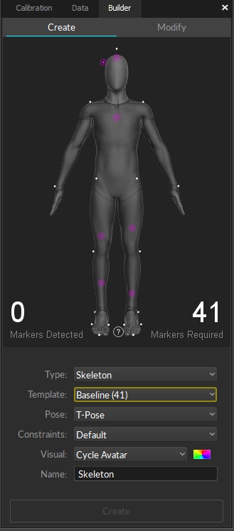
Open the Create tab on the .
From the Type drop-down list, select Skeleton.
Select a Marker Set to use from the drop-down menu. The number of required markers for each Skeleton is shown in parenthesis after the Marker Set name.
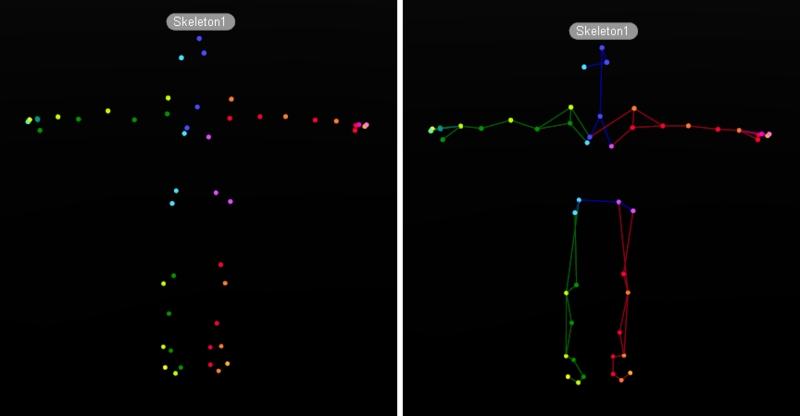
When a Marker Set is selected, the corresponding marker locations are displayed over an avatar in the . Right-drag to rotate the avatar to see the location of all the markers.
Have the subject strike a calibration pose (T-pose or A-pose) and carefully place retroreflective markers at the corresponding locations of the actor or the subject.
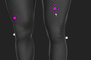
The positions of markers shown in white are fixed and must be in the same location for each skeleton created. These markers are critical in auto-labeling the skeleton.
The positions of markers shown in magenta are relative and should be placed in various positions in the general area to create skeletons that are unique to each actor.
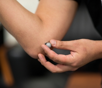
Joint markers need to be placed carefully along corresponding joint axes. Proper placements will minimize marker movements during a range of motions and will give better tracking results. To accomplish this, ask the subject to flex and extend the joint (e.g., knee) a few times and palpate the joint to locate the corresponding axis. Once the axis is located, attach the markers along the axis where skin movement is minimal during a range of motion.
Proper placement of Joint Markers improves auto-labeling and reduces post-production processing time.
Segment markers are placed on Skeleton body segments, but not around a joint. For best tracking results, place segment markers asymmetrically within each segment. This helps the Skeleton solve to thoroughly distinguish left from right for the corresponding Skeleton segments throughout the capture. This asymmetrical placement is also emphasized in the avatars shown in the Builder pane.
If attaching markers directly to skin, wipe off any moisture or oil before attaching the marker.
Avoid wearing clothing or shoes with reflective materials that can introduce extraneous reflections.
Tie up hair, which can occlude markers around the neck.
Remove reflective jewelry.
Place markers in an asymmetrical arrangement by offsetting the related segment markers (markers that are not on joints) at slightly different height.
The markers need to be placed on the skin for direct representation of the subject’s movement. Use appropriate adhesives to place markers and make sure they are securely attached.
Place markers where you can palpate the bone or where there is less soft tissue in between. These spots have fewer skin movements and provide more secure marker attachment.
Joint markers are vulnerable to skin movements because of the range of motion in the flexion and extension cycle. To minimize the influence, a thorough understanding of the biomechanical model used is necessary in the post-processing.
In certain circumstances, the joint line may not be the most appropriate location. Instead, placing the markers slightly superior to the joint line could minimize the soft tissue artifact, still taking care to maintain parallelism with the anatomical joint line.
Calibration markers exists only in the biomechanics Marker Sets.
Many Skeleton Marker Sets do not have medial markers because they can easily collide with other body parts or interfere with the range of motion, all of which increase the chance of marker occlusions.
However, medial markers are beneficial for precisely locating joint axes by associating two markers on the medial and lateral side of a joint. For this reason, some biomechanics Marker Sets use medial markers as calibration markers. Calibration markers are used only when creating Skeletons but removed afterward for the actual capture. These calibration markers are highlighted in red from the 3D view when a Skeleton is first created.
A proper calibration posture is necessary because the pose of the created Skeleton will be calibrated from it.
The avatar in the Builder pane does not change to reflect the selected pose.
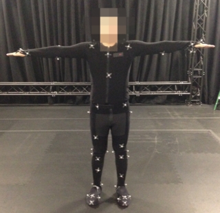
The T-pose is commonly used as the reference pose in 3D animation to bind two characters or assets together. Motive uses this pose when creating Skeletons. A proper T-pose requires straight posture with back straight and head facing directly forward. Both arms are parallel to the ground, forming a “T” shape, with the palms facing downward. Both arms and legs must be straight, and both feet need to be aligned parallel to each other.
The A-pose is especially beneficial for subjects who have restricted mobility in one or both arms. Unlike the T-pose, arms are abducted at approximately 40 degrees from the midline of the body, creating an A-shape. There are three different types of A-pose: Palms down, palms forward, and elbows bent.
Palms Down: Arms straight. Abducted, sideways, arms approximately 40 degrees, palms facing downwards.
Palms forward: Arms straight. Abducted, sideways, arms approximately 40 degrees, palms facing forward. Be careful not to over rotate the arm.
Elbows Bent: Similar to all other A-poses. arms approximately 40 degrees, bend elbows so that forearms point towards the front. Palms facing downwards, both forearms aligned.
Select the calibration Pose you plan to use to define the Skeleton from the drop-down menu. This is set to the T-pose by default.
Enter a unique name for the skeleton. The skeleton name is included as a prefix in the label for each of the skeleton markers.
Click Create. Once the Skeleton model has been defined, confirm all Skeleton segments and assigned markers are located at the expected locations. If any of the Skeleton segments seem to be misaligned, delete and create the Skeleton again after adjusting the marker placements and the calibration pose.
In Edit Mode
Reset Skeleton Tracking
When Skeleton tracking is not acquired successfully during the capture for some reason, you can use the CTRL + R hotkey to trigger the solver to re-boot the Skeleton asset.
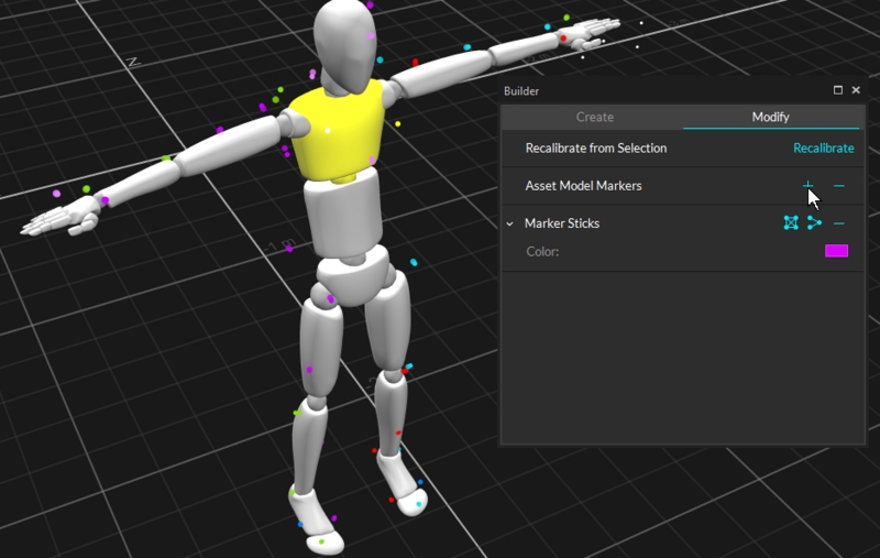
Several changes can be made to Skeleton assets from the Modify tab of the Builder pane, or through the context menus available in the 3D Viewport or the Assets Pane.
Post-Processing: Working with Recording Takes
Edit Mode is used for playback of captured Take files. In this mode, you can playback and stream recorded data and complete post-processing tasks. The Cameras View displays the recorded 2D data while the 3D Viewport represents either recorded or real-time processed data as described below.
There are two modes for editing:
Regardless of the selected Edit mode, you must reprocess the Take to create new 3D data based on the modifications made.
Skeleton assets can be recalibrated using the existing Skeleton information. Recalibration recreates the selected Skeleton using the same Skeleton Marker Set and refreshes expected marker locations on the assets.
There are several ways to recalibrate a Skeleton:
From the Modify tab of the Builder pane.
Select all of the associated Skeleton markers in the 3D Viewport, right-click and select Skeleton (1) --> Recalibrate from Selection.
Right-click the skeleton in the Assets pane and select Skeleton (1) --> Recalibrate from Markers.
Skeleton recalibration does not work for Skeleton templates with added markers.
Right-click the skeleton in the asset pane and select Constraints --> Reset Constraints to Default to update the Skeleton markers with the default constraints template.
Skeleton Marker Sets can be modified slightly by adding or removing markers to or from the template. Follow the below steps for adding/removing markers.
Modifying, especially removing, Skeleton markers is not recommended since changes to default templates may negatively affect the Skeleton tracking if done incorrectly.
Removing too many markers may result in poor Skeleton reconstructions, while adding too many markers may lead to labeling swaps.
If any modification is necessary, try to keep the changes minimal.
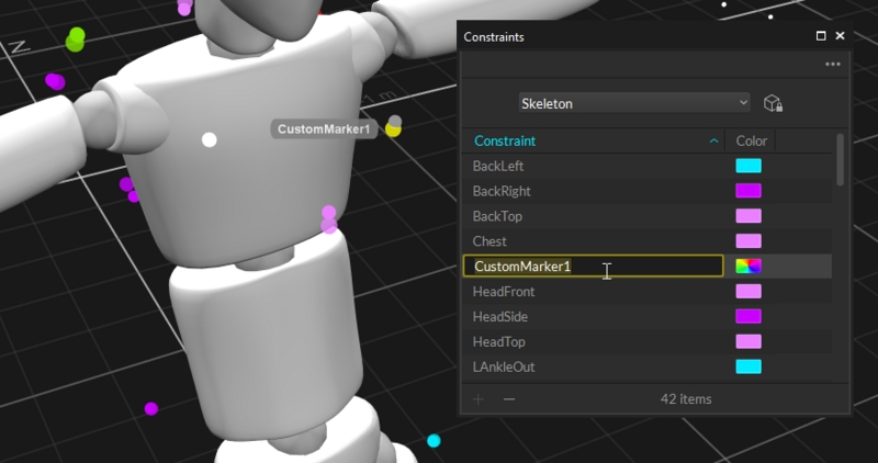
In the 3D Viewport, select the Skeleton segment that you are adding add the extra markers to.
CTRL + left-click on the marker that you wish to add to the skeleton.
You can also add Constraints from the Constraints pane.
Reconstruct and Auto-label the Take.
To Remove
[Optional] Under the advanced properties of the target Skeleton, enable the Marker to Constraint Lines property to view which markers are associated with different Skeleton bones.
Select the Skeleton segment to modify and the Marker Constraints you wish to dissociate.
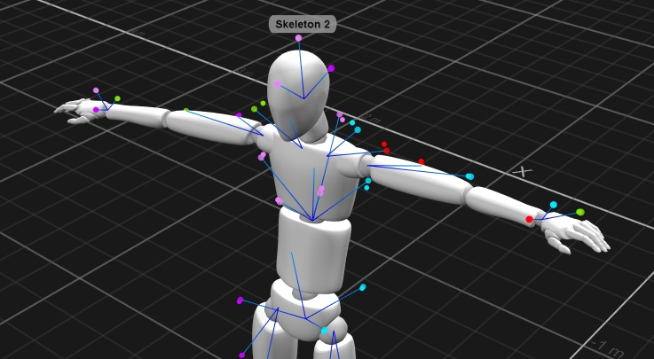
A Marker stick connects two markers to create a visible line. Marker sticks define the shape of an asset, showing which markers connect to each other, such as knee to hip, and which don't, such as hand to foot. Skeleton Marker Sets include the placement of marker sticks.
When asset definitions are exported to a MOTIVE user profile, the profile stores the marker arrangements calibrated in each asset, which can be imported into different takes without creating a new asset in Motive.
The user profile stores the spatial relationship of each marker to the others in the asset. Only the identical marker arrangement will be recognized and defined with the imported asset.
To export all of the assets in Live-mode or in the current TAKE file, go to File menu and selected Export Assets. You can also select the File menu → Export Profile option to export other software settings as well as the assets.
To export Skeleton constraints XML file
To import Skeleton constraints XML file
This page provides instructions for aligning a Rigid Body pivot point with a real object replicated 3D model.
When using streamed Rigid Body data to animate a real-life replicated 3D model, it's critical that the Rigid Body's pivot point aligns with the location of the pivot point in the corresponding 3D model. If they are not aligned, the animated motion will not be in a 1:1 ratio to the actual motion.
This alignment is critical for real-time VR applications where real-life objects are 3D modeled and animated in the scene.
These steps can be completed in Live or Edit mode.
There are two modes for editing:
Edit: Playback in standard Edit mode displays and streams the processed 3D data saved in the recorded Take. Changes made to settings and assets are not reflected in the Viewport until the Take is .
Edit 2D: Playback in Edit 2D mode performs a live reconstruction of the 3D data, immediately reflecting changes made to settings or assets. These changes are displayed in real-time but are not saved into the recording until the Take is and saved. To playback in 2D mode, click the Edit button and select Edit 2D.
Regardless of the selected Edit mode, you must reprocess the Take to create new 3D data based on the modifications made.
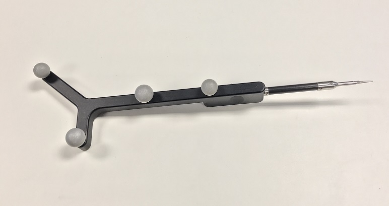
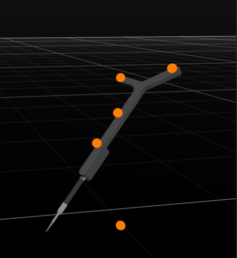
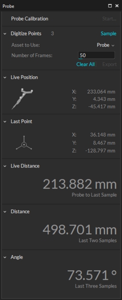
There are two methods to align the pivot point of a rigid body. We recommend using the measurement probe method as it is the most accurate.
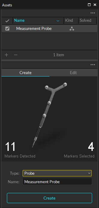
You can purchase an OptiTrack probe or create your own.
After generating 3D data points using the probe, attach the game geometry (obj file) to the Rigid Body.
Select the Rigid Body in either the Devices pane or the 3D Viewport to show its properties in the Properties pane.
In the Visuals section, select Custom Model under the Geometry property. (Note: this is an Advanced setting.)
This will open the Attached Geometry field. Click the folder to the right of the field to browse to the location of your 3D model.
From the sampled 3D points, You can also export markers created from the probe to Maya or other content creation packages to generate models guaranteed to scale correctly.
With both the Rigid Body and the 3D model selected, open the Modify tab in the Builder pane.
In the Align to... section, select Geometry.
The pivot point for the Rigid Body will snap to align with the pivot point for the 3D model.
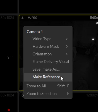
Use a reference camera when the option to use the probe method is not available.
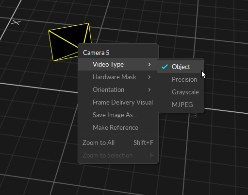
Change the Video Type for one of the cameras to grayscale mode.
Right-click the camera and select Make Reference.
This page provides detailed instructions on camera system calibration and information about the .
Calibration is essential for high quality optical motion capture systems. During calibration, the system computes the position and orientation of each camera and number of distortions in captured images to construct a 3D capture volume in Motive. This is done by observing 2D images from multiple synchronized cameras and associating the position of known calibration markers from each camera through triangulation.
If there are any changes in a camera setup the system must be recalibrated to accommodate those changes. Additionally, calibration accuracy may naturally deteriorate over time due to ambient factors such as fluctuations in temperature. For this reason, we recommend recalibrating the system periodically.
Prepare and optimize the capture volume for setting up a motion capture system.
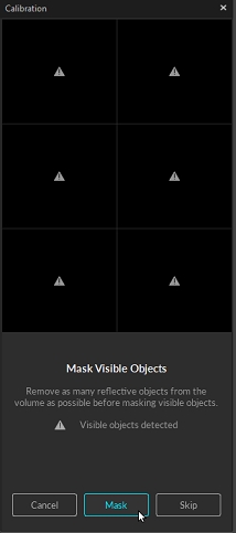
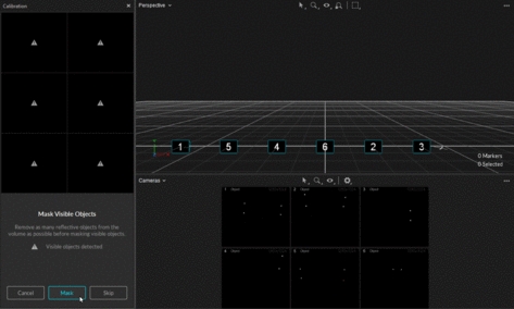
Apply masks to ignore existing reflections in the camera view.
Collect calibration samples through the wanding process.
Review the wanding result and apply calibration.
Set the ground plane to complete the system calibration.
Full: Calibrate all the cameras in the volume from scratch, discarding any prior known position of the camera group or lens distortion information. A Full calibration will also take the longest time to run.
Refine: Adjusts slight changes in the calibration of the cameras based on prior calibrations. This will solve faster than a Full calibration. Use this only if the cameras have not moved significantly since they were last calibrated. A Refine calibration will allow minor modifications in camera position and orientation, which can occur naturally from the environment, such as due to mount expansion.
Refinement cannot run if a full calibration has not been completed previously on the selected cameras.
Cameras need to be appropriately placed and configured to fully cover the capture volume.
Each camera must be mounted securely so that it remains stationary during capture.
Motive's camera settings used for calibration should ideally remain unchanged throughout the capture. Re-calibration may be required if there are any significant modifications to the settings that influence the data acquisition, such as camera settings, gain settings, and Filter Switcher settings.
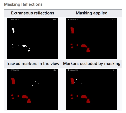
Before performing a system calibration, all extraneous reflections or unnecessary markers should be removed or covered so they are not seen by the cameras. When this isn't possible, extraneous reflections can be ignored by masking them in Motive.
Active Wanding:
Applying masks to camera views is only necessary when using calibration wands with passive markers. Active calibration wands calibrate the capture volume with the LEDs of all the cameras turned off. This method is recommended if the volume has a lot of reflective material that cannot be removed.
Check the corresponding camera view to identify where the reflection is coming from, and if possible, remove it from the capture volume or cover it for the calibration.
Masking from the Cameras Viewport
The wanding process is Motive's core pipeline for collecting calibration samples. A calibration wand with preset markers is waved repeatedly throughout the volume, allowing all cameras to see the calibration markers and capture the sample data points from which Motive will compute their respective position and orientation in the 3D space.
For best results, the following requirements should be met:
At least two cameras must see all three of the calibration markers simultaneously.
Cameras should see only calibration markers. If any other reflection or noise is detected during wanding the sample will not be collected and may affect the calibration results negatively. For this reason, the person doing the wanding should not be wearing anything reflective.
The markers on the calibration wand must be in good quality. If the marker surface is damaged or scuffed, the system may struggle to collect wanding samples.
There are different types of calibration wands suited for different capture applications. In all cases, Motive recognizes the asymmetrical layout of the markers as a wand and applies the dimensions of the wand selected at the beginning of the wanding process in calculating the calibration.
Unless specified otherwise, the wands use retro-reflective markers placed in a line at specific distances. For optimal results, it is important to keep the calibration wand markers untouched and undistorted.
Calibration Wands
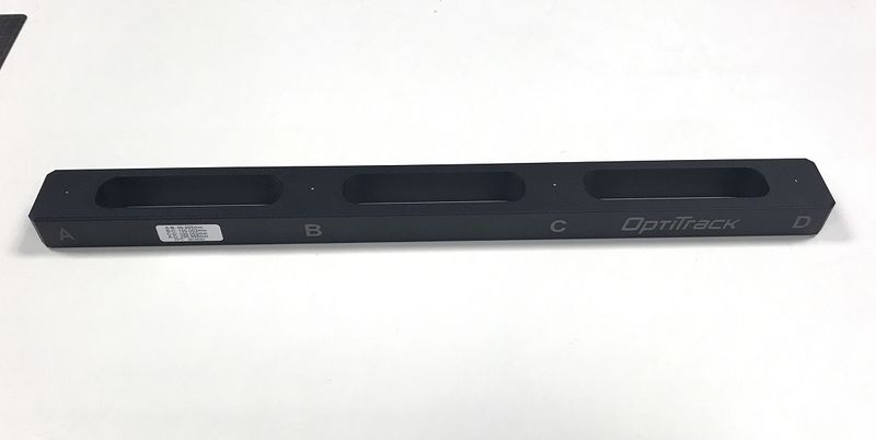
CW-500: The CW-500 calibration wand has a wand-width of 500mm when the markers are placed in configuration A. This wand is suitable for calibrating a large size capture volume because the markers are spaced farther apart, allowing the cameras to easily capture individual markers even at long distances.
CW-500 Active: With the same dimensions as the CW-500, the active wand is recommended for capture volumes that have a large amount of reflective material that cannot be removed. This wand calibrates the volume while the LEDs of all mounted cameras are turned off.
CW-250: The CW-250 calibration wand has a wand-width of 250mm. This wand is suitable for calibrating small to medium size volumes. Its narrower wand-width allows cameras in a smaller volume to easily capture all three calibration markers within the same frame. Note that a CW-500 wand can also be used like CW-250 wand if the markers are positioned in configuration B.
CWM-125 / CWM-250: Both CWM-125 and CWM-250 wands are designed for calibrating systems for precision capture applications. The accuracy of the calibrated wand width is the most precise and reliable on these wands, making them more suitable for precision capture in a small volume capture application.
To start calibrating inside the volume, cover one of the markers and expose it wherever you wish to start wanding. When at least two cameras detect all three markers and no other reflections in the volume, Motive will recognize the wand and will start collecting samples.
Confirm that masking was successful, and the volume is free of extraneous reflections. Return to the masking steps if necessary to mask any items that cannot be removed or covered.
To complete a full calibration, deselect any cameras that were selected during the previous steps so that no cameras are selected.
Set the Calibration Type. If you are calibrating a new capture volume, choose Full Calibration.
Under the Wand settings, specify the wand type you will use. Selecting the wrong wand type may result in scaling issues in Motive.
Double check the calibration setting. Once confirmed, press Start Wanding to start collecting wanding sample.
Bring your calibration wand into the capture volume and wave the wand gently across the entire volume. Slowly draw figure-eights repetitively with the wand to collect samples at varying orientations while covering as much space as possible for sufficient sampling.
Wanding Tips
Avoid waving the wand too fast. This may introduce bad samples.
Avoid wearing reflective clothing or accessories while wanding. This can introduce extraneous samples which can negatively affect the calibration result.
Try not to collect samples beyond 10,000. Extra samples could negatively affect the calibration.
Try to collect wanding samples covering different areas of each camera's view. The status indicator on Prime cameras can be used to monitor the sample coverage on individual cameras.
Although it is beneficial to collect samples all over the volume, it is sometimes useful to collect more samples in the vicinity of the target regions where more tracking is needed. By doing so, calibration results will have a better accuracy in the specific region.
Marker Labeling Mode
When performing calibration wanding, leave the Marker Labeling Mode at the default setting of Passive Markers Only. This setting is located in Application Settings → Live-Reconstruction tab → Marker Labeling Mode. There are known problems with wanding in one of the active marker labeling modes. This applies for both passive marker calibration wands and IR LED wands.
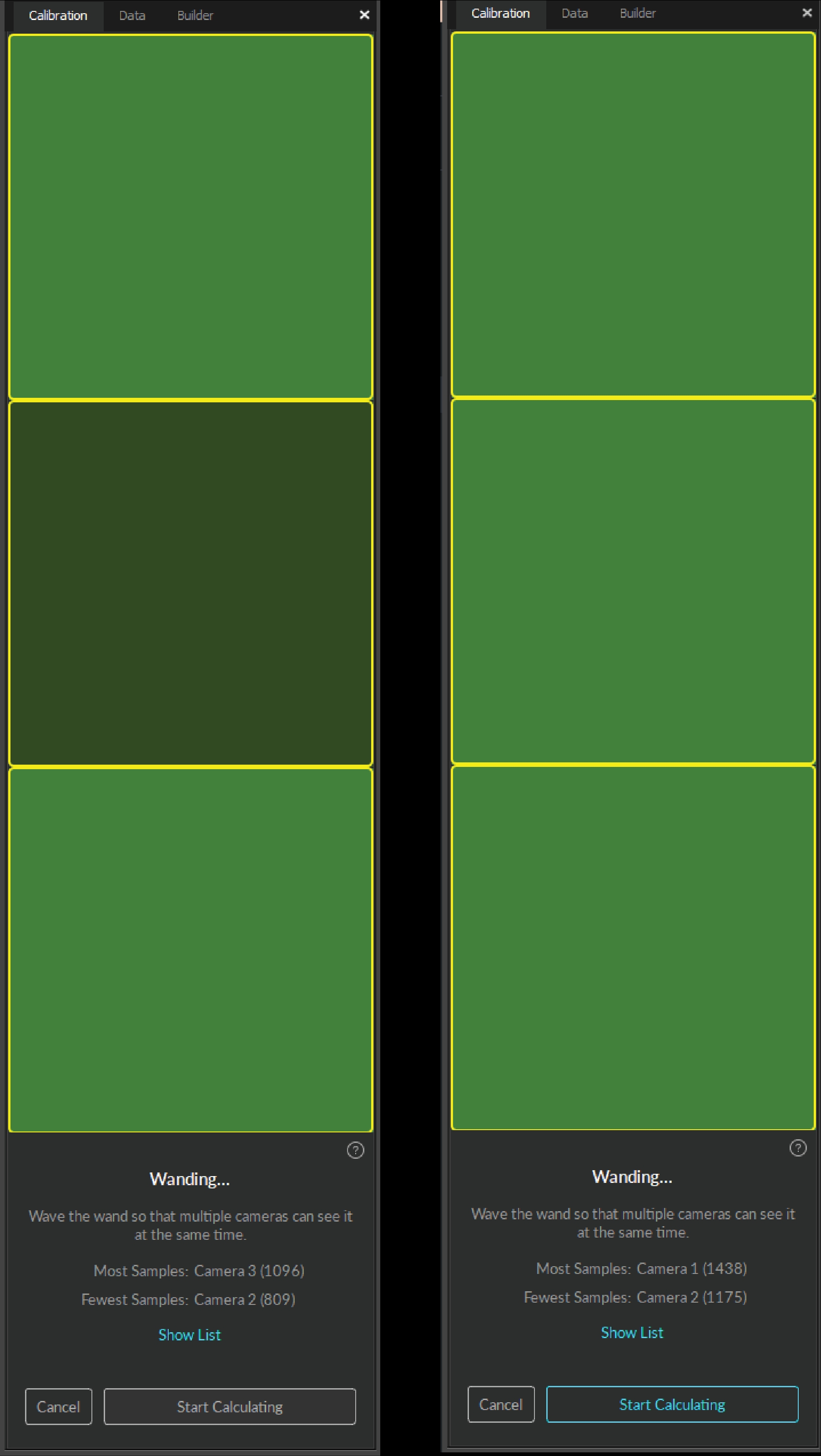
For Prime series cameras, the LED indicator ring displays the status of the wanding process.
When wanding is initiated, the LED ring turns dark.
When a camera detects all three markers on the calibration wand, part of the LED ring will glow blue to indicate that the camera is collecting samples. The location of the blue light will indicate the wand position in the respective camera view.
As calibration samples are collected by each camera, all the lights in the ring will turn green to indicate enough samples have been collected.
Cameras that do not have enough samples will begin to glow white as other cameras reach the minimum threshold to begin calibration. Check the 2D view to see where additional samples are needed.
When all of the cameras emit a bright green light to indicate enough samples have been collected, the Start Calculating button will become active.
Pess Start Calculating to calibrate. The length of time needed to calculate the calibration varies based on the number of cameras included in the system and the number of collected samples.
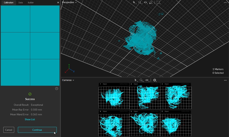
Click Show List to see the errors for each camera.
The result is determined by the mean error, resulting in the following ratings: Poor, Fair, Good, Great, Excellent, and Exceptional.
If the results are acceptable, press Continue to apply the calibration. If not, press Cancel and repeat the wanding process.
In general, if the results are anything less than Excellent, we recommend you adjust the camera settings and/or wanding techniques and try again.
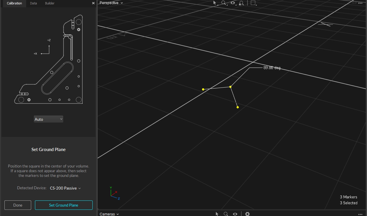
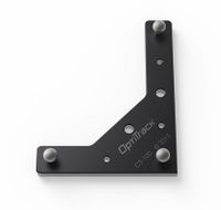
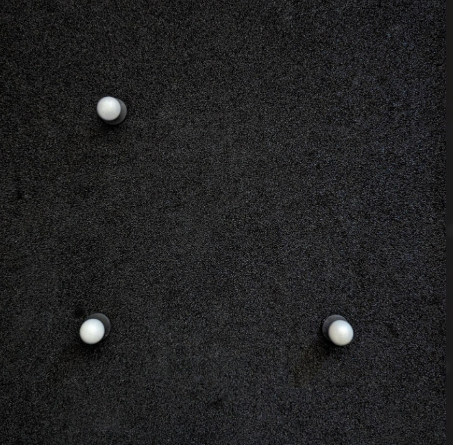
The final step of the calibration process is setting the ground plane and origin for the coordinate system in Motive. This is done using a Calibration Square.
Place the calibration square in the volume where you want the origin to be located, and the ground plane to be leveled.
If using a standard OptiTrack calibration square, Motive will recognize it in the volume and display it as the detected device in the Calibration pane.
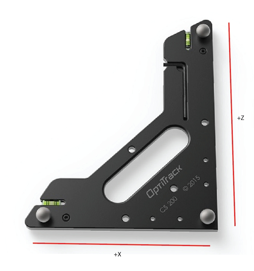
Align the calibration square so that it references the desired axis orientation. Motive recognizes the longer leg on the calibration square as the positive z axis, and the shorter leg as the positive x axis. The positive y axis will automatically be directed upward in a right-hand coordinate system.
Use the level indicator on the calibration square to ensure the orientation is horizontal to the ground. If any adjustment is needed, rotate the nob beneath the markers to adjust the balance of the calibration square.
If needed, the ground plane can be adjusted later.
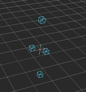
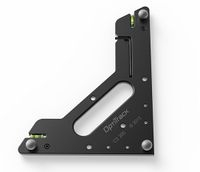
A custom calibration square can also be used to define the ground plane. All it takes to make a custom square is three markers that form a right-angle with one arm longer than the other, like the shape of the calibration square.
To use a custom calibration square, select Custom in the drop-down menu, enter the correct vertical offset and select the square's markers in the 3D Viewport before setting the ground plane.
Motive accounts for the vertical offset when using a standard OptiTrack calibration square, setting the origin at the bottom corner of the calibration square rather than the center of the marker.
When using a custom calibration square, measure the distance between the center of the marker and the lowest tip at the vertex of the calibration square. Enter this value in the Vertical Offset field in the Calibration pane.
The Vertical Offset property can also be used to place the ground plane at a specific elevation. A positive offset value will set the plane below the markers, and a negative value will set the plane above the markers.
To have the most control of the location of of the global origin, including placing it at the location of a marker, we recommend setting the origin to the pivot point of a rigid body.
Create the Rigid Body.
In the Calibration pane, select Rigid Body for the Ground Plane. Motive will set the origin to the selected Rigid Body's pivot point.
The Ground Plane Refinement feature improves the leveling of the coordinate plane. This is useful when establishing a ground plane for a large volume, because the surface may not be perfectly uniform throughout the plane.
To use this feature, place several markers with a known radius on the ground, and adjust the vertical offset value to the corresponding radius. Select these markers in Motive and press Refine Ground Plane. This will adjust the leveling of the plane using the position data from each marker.
To adjust the position and orientation of the global origin after the capture has been taken, use the capture volume translation and rotation tool.
To apply these changes to recorded Takes, you will need to reconstruct the 3D data from the recorded 2D data after the modification has been applied.
To rescale the volume, place two markers a known distance apart. Enter the distance, select the two markers in the 3D Viewport, and click Scale Volume.
Note: Whenever there is a change to the system setup (e.g. cameras moved) these calibration files will no longer be relevant and the system will need to be recalibrated.
Enabling/Disabling Continuous Calibration
When capturing throughout a whole day, temperature fluctuations may degrade calibration quality and create the need to recalibrate the capture volume at different times of the day. However, repeating the entire calibration process can be tedious and time-consuming especially for a system with a large number of cameras.
Instead of repeating an entire full calibration, you can record Takes while wanding and takes with the calibration square in the volume and use those takes to re-calibrate in the post-processing. This saves calibration calculation time on the capture day because you can apply the calibration from the recorded wanding take in the post-processing instead. Offline calibration allows time to inspect the collected capture data, re-calibrating from a recorded Take only when signs of degraded calibration quality are seen in the captures.
Capture wanding and ground plane Takes. At different times of the day, record wanding Takes that resemble the calibration wanding process. Also record corresponding ground plane Takes with the calibration square set in the volume to define the ground plane.
Whenever a system is calibrated, Motive saves two Calibration (*.cal) files, one of the Wanding and one of the Ground Plane. These files can be reloaded as needed and can also be used to complete an offline calibration.
Open the Take to be recalibrated.
Browse to and select the wanding Take that was captured around the same time as the Take to be recalibrated.
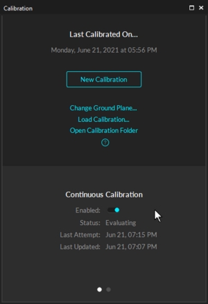
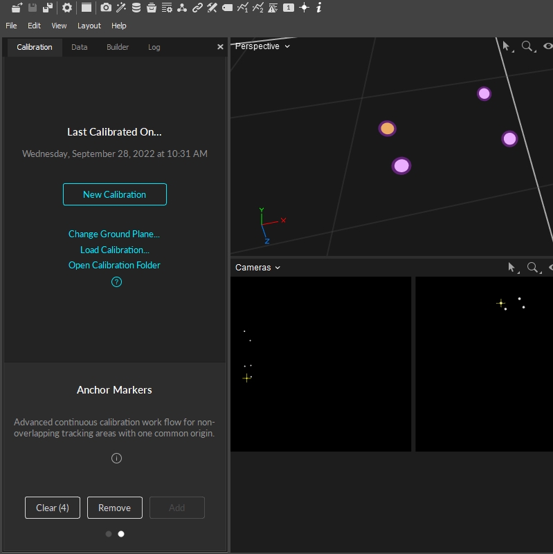
From the Calibration pane, click New Calibration.
In Edit mode, click Start Wanding. Motive will import the wanding from the Take file selected in step 3 and display the results.
Click the Start Calculating button.
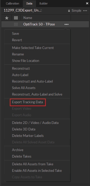
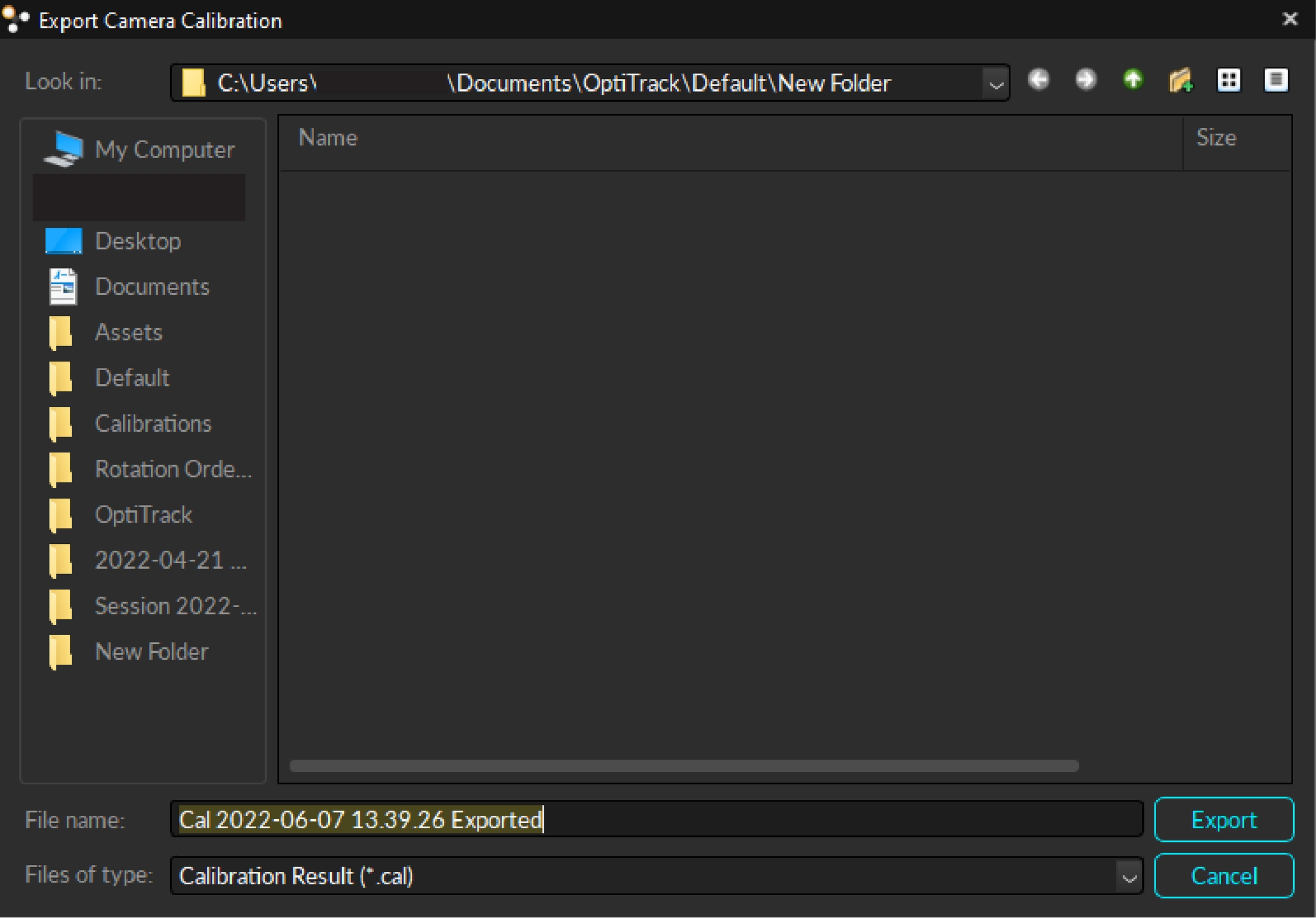
(Optional) Export the calibration results by selecting Export Camera Calibration from the File menu. The results will be saved as s .cal file.
Click Apply Results to accept the calibration.
Motive will move to the next step in the calibration process, setting the ground plane. If the ground plane is in a separate Take, then click Done and proceed to step 10. If the ground plane is in the calibration Take already loaded, then move to step 13.
From the Calibration pane, click Load Calibration...
Browse to and select the Ground Plane Take that was captured around the same time as the Take to be recalibrated.
From the Calibration pane, click Change Ground Plane.
Motive will display a warning that any 3D data in the take will need to be reconstructed and auto-labeled. Click Continue to proceed.
Partial calibration updates the calibration for selected cameras in a system by updating their position relative to the already calibrated cameras. Use this feature:
In a high camera count systems where only a few cameras need to be adjusted.
To recalibrate the volume without resetting the ground plane. Motive will retain the position of the ground plane from the unselected cameras.
To add new cameras into a volume that has already been calibrated.
Select the camera(s) to be recalibrated in the Cameras Viewport.
Select the Calibration Type. In most cases you will want to set this to Full, such as when adding new cameras to a volume or adjusting several cameras. When the camera moved slightly, Refine works as well.
Specify the wand type.
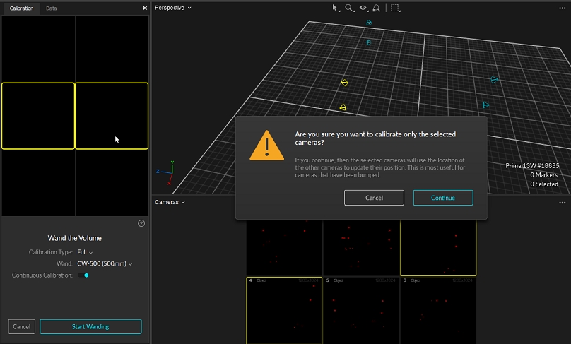
From the Calibration Pane, click Start Wanding. A warning message will ask you to confirm that only the selected cameras will be calibrated. Click continue.
Wand in front of the selected cameras and at least one unselected camera. This will allow Motive to align the cameras being calibrated with the rest of the cameras in the system.
When you have collected sufficient wand samples, click Calculate.
Click Apply. The selected cameras will now be calibrated to the rest of the cameras in the system.
Notes:
This feature requires the unselected cameras to be in a good calibration state. If the unselected cameras are out of calibration, using this feature will return bad calibration results.
Partial calibration does not update the calibration of the unselected cameras. However, the calibration report that Motive provides does include all cameras that received samples, selected or unselected.
Cameras can be modified using the gizmo tool if the Settings Window > General > Calibration > "Editable in 3D View" property is enabled. Without this property turned on the gizmo tool will not activate when a camera is selected to avoid accidentally changing a calibration. The process for using the gizmo tool to fix a misaligned camera is as follows:
Select the camera you wish to fix, then view from that camera (Hotkey: 3).
Select either the Translate or Rotate gizmo tool (Hotkey: W or E).
Use the red diamond visual to align the unlabeled rays roughly onto their associated markers.
Right click and choose Correct Camera Position/Orientation. This will perform a calculation to place the camera more accurately.
The OptiTrack motion capture system is designed to track retro-reflective markers. However, active LED markers can also be tracked with appropriate customization. If you wish to use Active LED markers for capture, the system will ideally need to be calibrated using an active LED wand. Please contact us for more details regarding Active LED tracking.
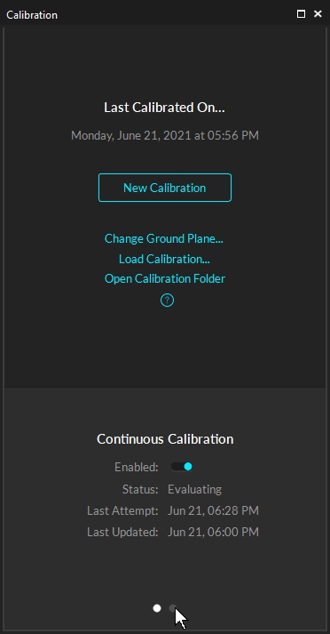
This page provides detailed information on the continuous calibration feature, which can be enabled from the . For additional Continuous Calibration features, please see the page.
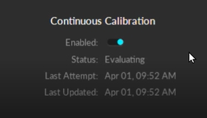
The Continuous Calibration feature ensures your system always remains optimally calibrated, requiring no user intervention to maintain the tracking quality. It uses highly sophisticated algorithms to evaluate the quality of the calibration and the triangulated marker positions. Whenever the tracking accuracy degrades, Motive will automatically detect and update the calibration to provide the most globally optimized tracking system.
Ease of use. This feature provides much easier user experience because the capture volume will not have to be re-calibrated as often, which will save a lot of time. You can simply enable this feature and have Motive maintain the calibration quality.
Optimal tracking quality. Always maintains the best tracking solution for live camera systems. This ensures that your captured sessions retain the highest quality calibration. If the system receives inadequate information from the environment, the calibration with not update and your system never degrades based on sporadic or spurious data. A moderate increase in the number of real optical tracking markers in the volume and an increase in camera overlap improves the likelihood of a higher quality update.
Works with all camera types. Continuous calibration works with all OptiTrack camera models.
For continuous calibration to work as expected, the following criteria must be met:
Markers Must Be Tracked. Continuous calibration looks at tracked reconstructions to assess and update the calibration. Therefore, at least some number of markers must be tracked within the volume.
Majority of Cameras Must See Markers. A majority of cameras in a volume needs to receive some tracking data within a portion of their field of view in order to initiate the calibration process. Because of this, traditional perimeter camera systems typically work the best. Each camera should additionally see at least 4 markers for optimal calibration. If not all the cameras see the markers at the same time, anchor markers will need to be set up to improve the calibration updates.
Anchor markers further improve the continuous calibration. When properly configured, anchor markers establish a known point-of-reference for continuous calibration updates, especially on systems that consists of multiple sets of cameras that are separated into different tracking areas, by obstructions or walls, without camera view overlap. Anchor markers provide extra assurance that the global origin will not shift during each update, which the continuous calibration feature checks for as well.
Active markers are best to use for anchors due to their unique active IDs, which improve accuracy, remove ambiguity, and enhance continuous calibration all around.
Cameras will always correctly identify an active marker even when no other markers are visible or after an occlusion. This helps the system calibrate more frequently, and to quickly adjust after more significant disturbances.
Anchor markers are critical to maintaining a single calibration throughout a partitioned volume. Active markers ensure that the cameras can correctly identify each anchor marker location.
Active markers allow bumped cameras to update faster and more accurately, and to recover from larger disturbances than passive markers.
For continuous calibration to work, It's important to have multiple markers visible to each camera, dispersed across a significant portion of that camera's field of view. This allows the system to more accurately determine the position and angle of the camera. This is true whether using active or passive markers.
Follow the steps below for setting up the anchor marker in Motive:
Adding Anchor Markers in Motive
Place any number of markers in the volume to assign them as the anchor markers.
Make sure these markers are securely fixed in place within the volume. It's important that the distances between these markers do not change throughout the continuous calibration updates.
In the 3D viewport, select the markers that are going to be assigned as anchors.
Click on Add to add the selected markers as anchor markers.
Once markers are added as anchor markers, magenta spheres will appear around the markers indicating the anchors have been set.
Add more anchors as needed, again, it's important that these anchor markers do not move throughout the tracking. Also when the anchor markers need to be reset, whether if the marker was displaced, you can clear the anchor markers and reassign them.
For multi-room setups, it is useful to group cameras into partitions. This allows for Continuous Calibration to run in each individual room without the need for camera view overlap.
From the Properties pane of a camera you can assign a Partition ID from the advanced settings.
You'll want to assign all the cameras in the same room the same Partition ID. Once assigned these cameras will all contribute to Continuous Calibration for their particular space. This will help ensure the accuracy of Continuous Calibration for each individual space that is a part of the whole system.
Within the Info Tab, you'll find additional Continuous Calibration features in order to update your Calibrations in real-time.
Below you'll find the steps for each of these features.
Camera Samples is a visual aid that shows which cameras may need more marker samples or a better distribution of marker samples.
Camera buttons within the Camera Samples section allow you to select the camera. This will also select the camera in the 2D Camera Viewport and Devices pane.
Markers within the field of view that are receiving good tracking rays will appear with a green diamond encompassing the marker.
Markers outside of the FOV will appear standard white.
Markers within FOV that have untracked rays will appear with a red diamond encompassing the marker.
If a camera appears under More Markers:
Select the camera under More Markers.
Navigate to the 2D Viewport and from the top left dropdown select "From Camera 'x'".
This will show the camera's field of view and any markers that it can see within the cyan box.
Add additional markers within the camera's view until the camera button is removed from More Markers.
You may have enough markers so that there are no cameras listed under More Markers, but still see cameras under Better Distribution.
Select a camera listed under Better Distribution.
Navigate to the 2D Viewport and from the top left dropdown select "From Camera 'x'".
This will show the camera's field of view and any markers that it can see within the cyan box.
Add additional markers that are more evenly distributed within the camera's view.
For Better Distribution, oftentimes all you need is a single additional marker separated from another cluster of markers as seen in the image above.
Anchor markers can be set up in Motive to further improve continuous calibration. When properly configured, anchor markers improve continuous calibration updates, especially on systems that consists of multiple sets of cameras that are separated into different tracking areas, by obstructions or walls, without camera view overlap. It also provides extra assurance that the global origin will not shift during each update, although the continuous calibration feature itself already checks for this.
The Anchor Markers section allows you to add/remove and import/export Anchor markers. It also shows the mean error under the Distance column for each individual Anchor marker and the overall in the top right in millimeters.
When the icon in the top right is a green circle with a check this denotes that all Anchor markers are visible by at least one camera.
When the icon is a red circle with an x this denotes that at least one Anchor is occluded from all cameras.
For multi-room setups, it is useful to group cameras into partitions. This allows for Continuous Calibration to run in each individual room without the need for camera view overlap.
The Partitions section directly corresponds with Partitions created in the Properties pane for each individual camera. This section displays the status of Continuous Calibration for each partition.
If a Partition or Partitions are not receiving enough marker data to validate or update, they will appear magenta in the table and a red circle with an x icon will appear in the top right of the section.
This is the Partition ID assigned via the camera's Properties pane. By default this value is 1.
Idle - Continuous Calibration is either turned off or there are not enough markers for Continuous Calibration to begin sampling.
Sampling - Continuous Calibration is collecting marker samples.
Evaluating - Continuous Calibration is determining if the latest samples are better than the previous and will update if necessary.
Processing - Processing will occur when an update is processing.
Last Validated will update its timestamp to 0h 0m 0s when the samples have been collected and the calibration solution was not deemed to be better than the solution already in place.
Last Updated will update its timestamp to 0h 0m 0s when good samples were collected and the calibration solution was deemed better than the solution in place.
This is the mean ray error for each partition in millimeters. The overall mean ray error will be displayed in the top right corner of the section.
This column denotes the number of Anchor markers that are visible within a partition.
The Partitions settings can be updated to custom values based on an individual user's needs. This ensures that the user is alerted when Continuous Calibration is not validating or updated. When these values are changed the Partitions section rows will turn magenta if they do not meet the standards of Maximum Error and/or Maximum Last Updated.
This setting can be changed to any positive decimal. If the ray error for a Partition exceeds this value, the text in the Partition's row will change to magenta and the icon on the top right of the Partition section will display a red circle with an 'x'.
Maximum Last Updated dictates how long Continuous Calibration can go without an update before the user is alerted (by a magenta text and a red circle with an 'x' icon) that Continuous Calibration has not been updated.
The Bumped Cameras features corrects a camera's position in Motive if it is physically bumped in the real 3D space.
Bumped Cameras needs to be enabled in the Info pane when initializing Continuous Calibration for any fixes to be applied. If it is NOT enabled and a camera is physically displaced, you will need to run a full Calibration to ensure accurate tracking.
Enable Bumped Cameras from the Bumped Cameras Settings:
Select Camera Samples for Mode.
Select either Anchor Markers, Active Markers, or Both from Marker Type.
Bumped Cameras is now able to correct physical camera movement without needing a full Calibration.
To see the results of Bumped Cameras steps above you can do the following:
The steps below are not necessary, but something you can do to see Bumped Cameras work in action.
Select the camera's view you intend to physically move in the 2D Camera Viewport.
Make sure Tracked and Untracked Rays are visible from the 'eye' icon in the 2D Camera Viewport.
Physically move the camera so that the markers appear with a red diamond around them (untracked).
Wait a few seconds and notice the camera's view shift to correct in the 2D Camera Viewport.
The red diamonds should now be green.
Disabled - When Mode is set to Disabled, Bumped Camera correction will not apply.
Camera Samples - When Mode is set to Camera Samples, Bumped Camera correction will correct based on the Camera Samples data. If Camera Samples is populated with cameras this will trigger Bumped Cameras to correct any cameras that may have moved. If a camera has NOT moved, this camera will remain idle in the Bumped Camera section until Camera Samples is clear of needed samples or distribution.
Selected Cameras - When Mode is set to Selected Cameras, this will ONLY correct the camera that is selected by the user from either the Devices, 3D or 2D viewport, or Camera Samples.
A camera MUST be selected during a bump for Selected Cameras mode to correct the camera's position.
It must also be de-selected after the camera posistion has been corrected, else the feature will continue to consume high CPU resources and left long term could have a negative effect in quality tracking.
Anchor Markers - ONLY Anchor Markers will be used to collect data for Bumped Cameras to correct a camera's position.
Active Markers - ONLY Active Markers will be used to collect data for Bumped Cameras to correct a camera's position.
Anchor and Active - BOTH Anchor and Active Markers will be used to collect data for Bumped Cameras to correct a camera's position.
If you only wish to have a few cameras corrected you can lower the count of the Max Camera Count. By default this is set to 20.
This page provides detailed instructions to create rigid bodies in Motive, and covers other useful features associated with rigid body assets.
In Motive, Rigid Body assets are used for tracking rigid, unmalleable, objects. A set of markers is securely attached to tracked objects, and respective placement information is used to identify the object and report 6 Degree of Freedom (6DoF) data. Thus, it's important that the distances between placed markers stay the same throughout the range of motion. Either passive retro-reflective markers or active LED markers can be used to define and track a Rigid Body.
A Rigid Body in Motive is a collection of three or more markers on an object that are interconnected to each other with an assumption that the tracked object is unmalleable. More specifically, Motive assumes the spatial relationship among the attached markers remains unchanged and the marker-to-marker distance does not deviate beyond the allowable tolerance defined under the corresponding Rigid Body properties. Otherwise, involved markers may become . Cover any reflective surfaces on the Rigid Body with non-reflective materials and attach the markers on the exterior of the Rigid Body where cameras can easily capture them.
Tip: If you wish to get more accurate 3D orientation data (pitch, roll, and yaw) of a Rigid Body, it is beneficial to spread markers as far as you can within the same Rigid Body. By placing the markers this way, any slight deviation in the orientation will be reflected from small changes in the position.
In a 3D space, a minimum of three coordinates are required for defining a plane using vector relationships. Likewise, at least three markers are required to define a Rigid Body in Motive. Whenever possible, it is best to use 4 or more markers to create a Rigid Body. Additional markers provide more 3D coordinates for computing positions and orientations of a rigid body, making overall tracking more stable and less vulnerable to marker occlusions. When any of markers are occluded, Motive can reference other visible markers to solve for the missing data and compute the position and orientation of the rigid body.
However, placing too many markers on one Rigid Body is not recommended. When too many markers are placed in close vicinity, markers may overlap on the camera view, and Motive may not resolve individual reflections. This can increase the likelihood of label-swaps during capture. Securely place a sufficient number of markers (usually less than 10), just enough to cover the main frame of the Rigid Body.
Tip: The recommended number of markers per Rigid Body is 4 ~ 12 markers.
You may encounter limits if using an excessive number of markers, or experience system performance issues when using the refine tool on such an asset.
Within a Rigid Body asset, the markers should be placed asymmetrically because this provides a clear distinction of orientations. Avoid placing the markers in symmetrical shapes such as squares, isosceles, or equilateral triangles. Symmetrical arrangements make asset identification difficult and may cause the Rigid Body assets to flip during capture.
When tracking multiple objects using passive markers, it is beneficial to create unique Rigid Body assets in Motive. Specifically, you need to place retroreflective markers in a distinctive arrangement between each object, which will allow Motive to more clearly identify the markers on each Rigid Body throughout capture. In other words, their unique, non-congruent, arrangements work as distinctive identification flags among multiple assets in Motive. This not only reduces processing loads for the Rigid Body solver, but it also improves the tracking stability. Not having unique Rigid Bodies could lead to labeling errors especially when tracking several assets with similar size and shape.
Note for Active Marker Users
The key idea of creating unique Rigid Body is to avoid geometrical congruency within multiple Rigid Bodies in Motive.
Unique Marker Arrangement. Each Rigid Body must have a unique, non-congruent, marker placement creating a unique shape when the markers are interconnected.
Unique Marker-to-Marker Distances. When tracking several objects, introducing unique shapes could be difficult. Another solution is to vary Marker-to-marker distances. This will create similar shapes with varying sizes and make them distinctive from the others.
Unique Marker Counts Adding extra markers is another method of introducing uniqueness. Extra markers will not only make the Rigid Bodies more distinctive, but they will also provide more options for varying the arrangements to avoid the congruency.
Having multiple non-unique Rigid Bodies may lead to mislabeling errors. However, in Motive, non-unique Rigid Bodies can also be tracked fairly well as long as the non-unique Rigid Bodies are continuously tracked throughout capture. Motive can refer to the trajectory history to identify and associate corresponding Rigid Bodies within different frames.
Depending on the object, there could be limitations on marker placements and number of variations of unique placements that could be achieved. The following list provides sample methods for varying unique arrangements when tracking multiple Rigid Bodies.
Create Distinctive 2D Arrangements. Use distinctive, non-congruent, marker arrangements as the starting point for producing multiple variations, as shown in the examples above.
Vary marker height. Use marker bases or posts of different heights to introduce variations in elevation to create additional unique arrangements.
Vary Maximum Marker to Marker Distance. Increase or decrease the overall size of the marker arrangements.
Add Two (or more) Markers Lastly, if an additional variation is needed, add extra markers. We recommended adding at least two extra markers in case any become occluded.
In creating a Rigid Body asset, a set of markers attached to a rigid object are grouped and auto-labeled as a Rigid Body. This Rigid Body definition can be used in multiple takes to continuously auto-label the same asset markers. Motive recognizes the unique spatial relationship in the marker arrangement and automatically labels each marker to track the Rigid Body.
Step 3: Click Create to define a Rigid Body asset from the selected markers.
You can also create a Rigid Body by doing the following actions while the markers are selected:
Perspective View (3D viewport): Right-click the selection in the perspective view to access the context menu. Under the Markers section, click Create Rigid Body.
Hotkey: While the markers are selected, use the create Rigid Body hotkey (Default: Ctrl +T).
Defining Assets in Edit mode:
There are multiple ways to add or remove markers on a Rigid Body.
Select the Modify tab.
The location of a pivot point can be adjusted by assigning it to a marker or by translating along the Rigid Body axis (x, y, z). For the most accurate pivot point location, attach a marker at the desired pivot location, set the pivot point to the marker, and apply the translation for precise adjustments.
Edit Mode is used for playback of captured Take files. In this mode, you can playback and stream recorded data and complete post-processing tasks. The Cameras View displays the recorded 2D data while the 3D Viewport represents either recorded or real-time processed data, as described below.
There are two modes for editing:
Regardless of the selected Edit mode, you must reprocess the Take to create new 3D data based on the modifications made.
Use the Location tool to enter the amount of translation (in mm) to apply along the (x, y, z) coordinates then click Apply. Clicking Apply again will add to the existing translation and can be used to fine-tune the adjustment of the bone.
Click Clear to reset the fields to 0mm.
Reset will position the pivot point at the geometric center of the Rigid Body according to its marker positions.
Use this tool to apply rotation to the local coordinate system of a selected Rigid Body. You can also reset the orientation to re-align the Rigid Body coordinate axis and the global axis. When resetting the orientation, the Rigid Body must be tracked in the scene.
In addition to the Reset buttons on the Builder pane, you can right-click a selected rigid body to open the Asset(s) context menu. Select Bones (#) --> Reset Location.
The Align to Geometry feature provides an option to align the pivot of a rigid body to a geometry offset. Motive includes several standard geometric objects that can be used, as well as the ability to import custom objects created in other applications. This allows for consistency between Motive and external rendering programs such as Unreal Engine and Unity.
Scroll to the Visuals section of the asset's properties. Under Geometry, select the object type from the list.
To import your own object, select Custom Model. This will open the Attached Geometry field. Click on the file folder icon to select the .obj or .fbx file to import into Motive.
To align an asset to a specific camera, select both the asset and the camera in the 3D ViewPort. Click Camera in the Align to... field in the Modify tab.
To align an asset to an existing Rigid Body, you must be in 2D edit mode. Click the Edit button at the bottom left and select EDIT 2D from the menu.
This feature is useful when tracking a spherical object (e.g., a ball). Motive will assume all of the markers on the selected Rigid Body are placed on the surface of a spherical object and will calculate and re-position the pivot point accordingly. Simply select a Rigid Body in Motive, open the Builder pane to edit Rigid Body definitions, and then click Apply to place the pivot point at the center of the spherical object.
The Rigid Body refinement tool improves the accuracy of the Rigid Body calculation in Motive. When a Rigid Body asset is initially created, Motive references only a single frame to define it. The Rigid Body refinement tool allows Motive to collect additional samples, achieving more accurate tracking results by improving the calculation of expected marker locations of the Rigid Body as well as the position and orientation of the Rigid Body itself.
Click the Modify tab.
Select the Rigid Body to be refined in the Asset pane.
In the Refine section of the Modify tab of the Builder pane, click Start...
Slowly rotate the Rigid Body to collect samples at different orientations until the progress bar is full.
You can also refine the asset in Edit mode. Motive will automatically replay the current take file to complete the refinement process.
Select Tool (Hotkey: Q): The Default option. Used for selecting objects in the Viewport. Return to this mode when you are done using the Gizmo tools.
Translate Tool (Hotkey: W): Translate tool for moving the Rigid Body pivot point.
Rotate Tool (Hotkey: E): Rotate tool for reorienting the Rigid Body coordinate axis.
Scale Tool (Hotkey: R): Scale tool for resizing the Rigid Body pivot point.
Rigid Body tracking data can be exported or streamed to client applications in real-time:
You can disable assets and hide their associated markers once you are finished labeling and editing them to better focus on the remaining unedited assets.
To Hide Markers:
Select Markers > Hide for Disabled Assets.
When an asset definition is exported to a user profile, Motive stores marker arrangements calibrated to the asset, which allows the asset to be imported into different takes without being rebuilt each time in Motive.
Profile files specifically store the spatial relationship of each marker. Only the identical marker arrangements will be recognized and defined with the imported asset.
To export all of the assets in Live or in the current TAKE file, go to the File menu → Export Assets.
You can also select Export Profile from the File menu to export other software settings, in addition to the assets.
Trained Markersets allow you to create Assets from any object that is not a Rigid Body or a pre-defined Skeleton. This allows you to track anything from a jump rope, to a dog, to a flag, to anything in between.
Please follow the steps below to get started.
In order to get the best training data, it is imperative to record markers with little to no occlusion and arrange markers asymmetrically. If you do have occlusions, it is important to fill in gaps using the Edit Tool in Edit mode.
Attach an adequate number of markers to your flexible object. This is highly dependent on the object but should cover at least the outline and any internal flex points. e.g., if it's a mat, the mat should have markers along the edges as well as dispersed markers in the middle in an asymmetrical pattern. If it's an animal or something that has real-life bones, try to add markers on either side of any joints just like you see on the Skeleton marker sets.
Record the movements you want of the object, trying to get as much of the full range of motion as possible.
In Edit mode, select the markers attached to the object.
Right-click and select Create Markerset.
Right-click the newly created asset and select Training -> Auto-Generate Asset.
To add Bones from the 3D viewport:
First make sure the Markerset is selected in the Assets pane, then hold down CTRL while selecting the markers from which you wish to make a bone.
Right click on one of the markers and select Bone(s) -> Add From Marker(s).
Tips for making bones:
Make sure the asset has enough markers to make all the bones track well.
Choose markers that are semi-rigid relative to one another when possible for bone constraints.
A bone can be made from one or more markers:
A bone made from 3+ markers will track with 6 Degrees of Freedom (DoF). Use this type of bone for end effectors and generally whenever possible.
A bone made from 2 markers will track with 5 Degrees of Freedom and a bone made from 1 marker will track with 3 Degrees of Freedom (only positional data). This means that rotational values may turn out strange if it is not connected to a 6 DoF bone on either end. This type is well-suited for under-constrained segments like an elbow with only one or two markers on it.
Once you are finished adding the necessary bones you can create Bone Chains to connect bones:
Select at least 1 bone (if you have multiple selected make sure the one you select first is the one you wish to make the first 'parent' bone then any subsequent children/parent bones should follow).
Right click in 3D viewport and select Bone(s) -> Add Bone Chain.
Solve your Markerset: right click on asset in asset pane and select Solve. You can now export, or stream, or do whatever else you'd like in Edit.
If you would like your Asset to be available in Live, simply right click on the Markerset in the Assets pane and select Copy Asset to Live.
And voilà, you have a Markerset you can track and record in Live.
This adds marker training and Auto-Generates Marker Sticks. This function only needs to be performed once after a Markerset has been created.
Add Marker Training goes through and adds a learned model of the Markerset. It's best to train the Markerset based on a full Range of Motion of the object you would like to track. This means moving the object to the limits of how it can move for one take, then labeling that take as well as you can, then running this training method on it.
Add the Training Count column to the Asset pane to show how many times you've used the Add Marker Training command on a Markerset.
This removes any marker training that was added either by Auto-Generate Asset or Add Marker Training. This is useful if you changed labels and wanted to reapply new marker training based on the new labels.
This automatically generates bones at flex points. This is why recording a full range of motion of your object is important so these bones can be added correctly.
This applies another round of Marker Training and refines Bone positions based on new training information.
This applies another round of Marker Training and refines Constraint positions based on new training information.
This is how you can create Bones manually from selected markers.
This removes the Bone from the Markerset and 3D viewport.
This adds a parent/child relationship to bones.
This removes the Bone Chain between bones.
When a child bone is selected, you can select Reroot Bones to make a child bone the parent. i.e. Bone 002 is a child of Bone 001 and Bone 001 (the root bone) is a child to Markerset 001. After selecting Bone 002 and Reroot bones, Bone 002 is now the parent to Bone 001 and the child to Markerset 001.
This will align the selected Bone to a selected camera.
This will align the selected Bone to another selected Bone.
If the Bone position was altered by either the Gizmo Tool or by Align to Camera/Other Bone, you can reset its default position with Reset Location.
The active Session Folder is noted with a flag icon. To switch to a different folder, left-click the folder name in the Session list.
The Visual Aids menu allows you to select which data to display.
When needed, the Viewport can be split into 3 or 4 smaller views. Click the in the top-right corner of the viewport to open the Viewport context menu to select additional panes or different layouts. You can also use the hotkey Shift + 4 to open the four pane layout.
When needed, additional Viewer panes can be opened from the View menu or by clicking the icon on the main toolbar.
Mouse controls in Motive can be customized from the Mouse tab in application settings panel to match your preference. Motive also includes common mouse control presets for Motive (the default), Blade, Maya, MotionBuilder and Visual3D applications. Click the button to open the Settings panel.
Hotkeys speed up workflows. See all the defaults on the Motive Hotkeys page. To create custom hotkeys, save or import a keyboard preset, click the button to open the Settings panel.
The button at the far left of the Control Deck switches between Live and Edit mode, with the active mode shown in cyan. Hotkey Shift + ~ toggles between Live and Edit modes.
Right-click and drag on a graph to zoom in and out on both vertical and horizontal axis. If Autoscale Graph is enabled, the vertical axis range will be fixed according to the max and min values of the plotted data.
Enter the start and end frames of the working range in the fields in the Control Deck.
Access Application Settings from the Edit menu or by clicking the icon on the main toolbar. Read more about all of the available settings on the Application Settings pages.
Assets used in the current TAKE are displayed in and managed from the Assets pane. To open the Assets pane, click the icon.
The Vertical Offset is the distance between the center of the markers on the and the actual ground and is a required value in setting the global origin.
All markers need to be placed at respective anatomical locations of a selected Skeleton as shown in the . Skeleton markers can be divided into two categories: markers that are placed along joint axes (joint markers) and markers that are placed on body segments (segment markers).
In the Builder pane, the number of Markers Needed and Markers Detected must match. If the Skeleton markers are not automatically detected, manually select the Skeleton markers from the .
Find detailed descriptions of each template in the section .
require precise placement of markers at the respective anatomical landmarks. The markers directly relate to the coordinate system definition of each respective segment, affecting the resulting biomechanical analysis.
While the basic marker placement must follow the avatar in the Builder pane, additional details on the accurate placements can be found on the page.
After creating a Skeleton from the , calibration markers need to be removed. First, detach the calibration markers from the subject. Then, in Motive, right-click on the Skeleton in the perspective view to access the context menu and click Skeleton → Remove Calibration Markers. Check the to make sure that the Skeleton no longer expects markers in the corresponding medial positions.
Once the skeleton markers are for the selected template, it's time to finish creating the skeleton.
The Constraints drop-down allows you to assign labels that are defined by the Marker Set template (Default) or to assign custom labels by l file of constraint names.
Select the Visual template to apply to the skeleton. Options are: Segment; Avatar - male; Avatar - female; None; or Cycle Avatar, which cycles between the male and female avatars. This value can be changed later in the .
Ask the subject to stand in the selected , feet shoulder-width apart. The T-pose should be done with palms downward.
If you are creating a Skeleton in the post-processing of captured data, you will have to the Take to see the Skeleton modeled and tracked in Motive.
Skeleton marker colors and marker sticks can be viewed in the 3D Viewport. They provide color schemes for clearer identification of Skeleton segments and individual marker labels. To make them visible, enable Marker Sticks and Marker Colors under the visual aids in the pane.
Edit: Playback in standard Edit mode displays and streams the processed 3D data saved in the recorded Take. Changes made to settings and assets are not reflected in the Viewport until the Take is .
Edit 2D: Playback in Edit 2D mode performs a live reconstruction of the 3D data, immediately reflecting changes made to settings or assets. These changes are displayed in real-time but are not saved into the recording until the Take is and saved. To playback in 2D mode, click the Edit button and select Edit 2D.
Constraints store information on marker labels, colors, and marker sticks which can be modified, exported and re-imported as needed. For more information on exporting and importing constraints, please refer to the page.
To modify marker colors and labels, use the .
When adding, or removing, markers in the Edit mode, the Take needs to be again to re-label the Skeleton markers.
Open the Modify tab on the .
On the Marker Constraints tool in the Builder pane, click to add and associate the selected marker to the selected segment.
Extra markers added to Skeletons will be labeled as Skeleton_CustomMarker#. Use the to change the label as needed.
Enable selection of Marker Constraints from the visual aids option in .
Open the Modify tab on the .
Delete the association by clicking on the in the Constraints section.
Alternately, you can click to remove selected markers from the Constraints pane.
From the , right click the Take and select Reconstruct and Auto-label.
For newly created Skeletons, default Skeleton creation properties are configured under the . Click the button and select Assets.
Properties of existing, or recorded, Skeleton assets are configured under the while the respective Skeletons are selected.
To configure Advanced properties, click the button in the top right corner of the pane.
Assets can be exported into the Motive user profile (.MOTIVE file) if they need to be re-imported. The is a text-readable file that contains various configuration settings in Motive, including the asset definitions.
There are two ways of obtaining Skeleton joint angles. Rough representations of joint angles can be obtained directly from Motive, but the most accurate representations of joint angles can be obtained by pipelining the tracking data into a third-party biomechanics analysis and visualization software (e.g. or ).
For biomechanics applications, joint angles must be computed accurately using the respective Skeleton model solve, which can be accomplished by using biomechanical analysis software. or stream tracking data from Motive and import into an analysis software for further calculation. From the analysis, various biomechanics metrics, including the joint angles, can be obtained.
Joint angles generated and exported from Motive are intended for basic visualization purposes only and should not be used for any type of biomechanical or clinical analysis. A rough representation of joint angles can be obtained by either exporting or streaming the Skeleton Rigid Body tracking data. When exporting the tracking data into CSV, set the export setting to Local to obtain bone segment position and orientation values in respect to its parental segment, roughly representing the joint angles by comparing two hierarchical coordinate systems. When streaming the data, set to true in the streaming settings to get relative joint angles.
Each Skeleton asset has its marker templates stored in a Constraints XML file. A Skeleton Marker Set can be modified by exporting, customizing, and importing the Constraints XML files. Specifically, customizing the XML files will allow you to modify Skeleton marker labels, marker colors, and marker sticks within a Skeleton asset. For detailed instructions on modifying Skeleton XML files, read the page.
To export a Skeleton XML file, right-click on a Skeleton asset under the Assets pane and select Constraints --> to export corresponding Skeleton marker XML file.
When creating a new Skeleton, you can import a constraints XML file under the Labels section of the To import a constraints XML file to an existing Skeleton, right-click on a Skeleton asset under the Assets pane and select Constraints --> Import Constraints.
from the markers on the target object. By default, Motive will position the pivot point of the Rigid Body at the geometric center of the marker placements. Once the Rigid Body has been created, place the object in a stable location where it will remain stationary.
Please refer to page for instructions to create a measurement probe asset in Motive.
Use the created measurement probe to collect that outline the silhouette of the object. Mark all corners and other key features on the object.
Next, use the to translate the 3D model to align with the silhouette sample collected in Step 3. Move, rotate, and scale the model until it is perfectly aligned with the silhouette.
Decrease the size of the marker visual to improve accuracy when aligning the object. To change the marker size, click the button to open the Application Settings panel. Go to View -> 3D View -> Markers -> Custom Size.
This will create a Rigid Body overlay in the . Follow steps , , and above using the reference video to align the Rigid Body pivot.
Motive opens the calibration layout view by default, containing the necessary panes for the calibration process. This layout can also be accessed from the calibration layout button in the top-right corner, or by using the Ctrl+1 .
The will guide you through the calibration process. This pane can be accessed by clicking on the icon on the toolbar or by entering the calibration layout from the top-right corner . For a new system calibration, click the New Calibration button and Motive will walk you through the steps.
The default grid size for the 3D Viewport is 6 square meters. To change this to match the size of the capture volume, click the Settings button. On the Views / 3D tab, adjust the values for the Grid Width and Grid Length as needed.
When the cameras detect reflections in their view, it will be indicated with a warning sign to alert which cameras are seeing reflections; for Prime series cameras, the indicator LED ring will also light up in white.
Masks can be applied by clicking Mask in the , and it will apply red masks over all of the reflections detected in the 2D camera view. Once masked, the pixels in the masked regions will entirely be filtered out from the data. Please note that Masks get applied additively, so if there are already masks applied in the camera view, clear them out first before applying a new one.
The will display a warning for any cameras that see reflections or noise in their view.
In the , click Mask to apply masks over all reflections in the view that cannot be removed or covered, such as other cameras.
Masks can also be applied from the Cameras Viewport if needed. From the Cameras view, click the gear icon on the toolbar to see . You can also click on the icon to switch to to manually apply or erase masks.
Masked pixels are completely filtered from the , which means the data in masked regions will not be collected for computing the . For this reason, excessive use of masking may result in data loss or frequent marker occlusions.
Wanding trails will show in color in the for each camera. As you wand, consult the Cameras Viewport to evaluate individual camera coverage. Each camera should be thoroughly covered with wand samples (see image, below). If there are any large gaps, focus wanding on those areas to increase coverage.
The will display a table of the wanding status to monitor the progress. For best results, wand evenly and comprehensively throughout the volume, covering both low and high elevations.
Continue wanding until the camera squares in the turn from dark green (insufficient number of samples) to light green (sufficient number of samples). Once all the squares have turned light green the Start Calculating button will become active.
Press Start Calculating in the . Generally, 1,000-4,000 samples per camera are enough. Samples above this threshold are unnecessary and can be detrimental to a calibration's accuracy.
As Motive starts calculating, blue wanding paths will display in the view panes, and the will update with the calibration result from each camera.
Tip: Select a Take in the to see its related calibration results in the . This information is available only for Takes recorded in Motive 1.10 and above.
When the calculation is done the results will display in the .
Once the calibration square is properly placed and detected by the , click Set Ground Plane. You may need to manually select the markers on the ground plane if Motive fails to auto-detect the ground plane.
The Vertical Offset is the distance between the center of the markers on the and the actual ground and is a required value in setting the global origin.
Align the Rigid Body's pivot point to the location you would like to set as the global origin (0,0,0). To align the pivot point to a specific marker, shift-select the marker and the pivot point. From the , click the Modify tab and select Align to...Marker.
Select the Rigid Body in the before proceeding to set the ground plane.
On the main Calibration pane, Click Change Ground Plane... for additional tools to further refine your calibration. Use the page selector at the bottom of the pane to access the various page.
Calibration files are used to preserve calibration results. The information from the calibration is exported or imported via the CAL file format. Calibration files eliminate the effort of calibrating the system every time you open Motive. Calibration files are automatically saved into the default folders after each calibration. In general, we recommend exporting the calibration before each capture session. By default, Motive loads the last calibration file that was created. This can be changed via the .
The continuous calibration feature continuously monitors and refines the camera calibration to its best quality. When enabled, minor distortions to the camera system setup can be adjusted automatically without wanding the volume again. In other words, you can calibrate a camera system once and no longer worry about external distortions such as vibrations, thermal expansion on camera mounts, or small displacements on the cameras. For detailed information, read the page.
Continuous calibration is enabled from the once a system has been calibrated. It will also show when the continuous calibration last updated and its current status.
From the , click Load Calibration...
Select Custom for the ground plane type, enter the distance, select the three markers of the ground plane from the 3D Viewport, then click Change Ground Plane.
If is not enabled and a camera is bumped, use Partial Calibration to adjust the camera that is now out of place.
Open the and select New Calibration.
The Calibration Pane will display the . Repeat steps 2-7 until the results are Excellent or Exceptional.
Turn on if not already done. Continuous calibration should finish aligning the camera into the correct location.
A: This can occur if the capture volume was calibrated with the wrong selected, or if the volume was incorrectly .
If markers on the calibration wand have been damaged, please to have them replaced.
Live Mode Only. Continuous calibration only works in .
To enable Continuous Calibration, calibrate the camera system first and enable the Continuous Calibration setting at the bottom of the . Once enabled, Motive continuously monitors the residual values in captured marker reconstructions, and when the updated calibration is better than the existing one, it will get updated automatically. Please note that at least four (default) marker samples must be being tracked in the volume for the continuous calibration to work. You will also be able to monitor the sampling progress and when the calibration has been last updated.
Please see the page for additional features.
First, make sure the entire camera volume is fully and prepared for marker tracking.
Open the and select the second page at the bottom to access the anchor marker feature.
In the event that you need to manually adjust cameras in the 3D view, you can enable Editable in 3D View in . To access this setting, you'll need to select Show Advanced from the 3-dot more options dropdown at the top. This will populate a Calibration section on this window.
This allows you to use the to Translate, Rotate, and Scale cameras to their desired locations.
For additional information regarding Anchor markers, please see this .
For more information, please see the Partitions section .
Create Anchor markers from the section or add Active markers.
If you are using for tracking multiple Rigid Bodies, it is not required to have unique marker placements. Through the active labeling protocol, active markers can be labeled individually, and multiple rigid bodies can be distinguished through uniquely assigned marker labels. Please read through page for more information.
Even though it is possible to track non-unique Rigid Bodies, we strongly recommend making each asset unique. Tracking of multiple congruent Rigid Bodies could be lost during capture either by occlusion or by stepping outside of the capture volume. Also, when two non-unique Rigid Bodies are positioned in vicinity and overlap in the scene, their marker labels may get swapped. If this happens, additional efforts are required to in post-processing of the data.
Step 1: Select all associated Rigid Body markers in the .
Step 2: On the , confirm that the selected markers match those on the object you want to define as the Rigid Body.
Assets pane: Click the add button at the bottom of the .
Step 4: Once the Rigid Body asset is created, the markers will be colored (labeled) and interconnected to each other. The newly created Rigid Body will be listed under the .
Motive can detect and pair a rigid body to its associated IMU. See the page for more details.
If Rigid Bodies are created in Edit mode, the corresponding Take needs to be . The Rigid Body markers will be labeled using the Rigid Body asset and positions and orientations will be computed for each frame. If the 3D data have not been labeled after edits on the recorded data, the asset may not be tracked.
Rigid Body properties define the specific configurations of Rigid Body assets and how they are tracked and displayed in Motive. For more information on each property, read the page.
Default properties are applied to any newly created asset, such as minimum markers to boot or continue, asset scale, and asset name and color. Default properties are configured under the Assets section in the panel. Click the button to open.
Properties for existing Rigid Body assets can be changed from the .
From the , select the Rigid Body that needs markers added or removed.
In the 3D , select the marker(s) to be added or removed.
From the :
At the bottom of the pane, click to add or to remove the selected marker(s).
From the :
In the Marker Constraints section, click to add or to remove the selected marker(s).
The pivot point or bone of a Rigid Body is used to define both its position and orientation. The default position of the bone for a newly created rigid body is at its geometric center and its orientation axis will align with the global coordinate axis. To view the pivot point in the 3D viewport, enable the Bone setting in the Visuals section of the selected Rigid Body in the .
Position and orientation of a tracked Rigid Body can be monitored in real-time from the . Select a Rigid Body in Motive, open the Info pane by clicking the button on the toolbar. Click the button in the top right corner and select Rigid Bodies from the menu to view respective real-time tracking data of the selected Rigid Body.
Edit: Playback in standard Edit mode displays and streams the processed 3D data saved in the recorded Take. Changes made to settings and assets are not reflected in the Viewport until the Take is .
Edit 2D: Playback in Edit 2D mode performs a live reconstruction of the 3D data, immediately reflecting changes made to settings or assets. These changes are displayed in real-time but are not saved into the recording until the Take is and saved. To playback in 2D mode, click the Edit button and select Edit 2D.
By default, the orientation axis of a Rigid Body is aligned with the global axis when the Rigid Body is first created. Once it's created, its orientation can be adjusted, either by editing the Rigid Body orientation through the or by using the GIZMO tools.
Several tools are available on the Builder pane to align Rigid Bodies. Click to open the builder pane then click on the Modify tab. Select a Rigid Body in the 3D Viewport to see the Rigid Body tools.
To use this feature, select the rigid body from the Assets pane. In the Properties pane, click the button and select Show Advanced if it is not already selected.
From the menu, open the , or click the button on the toolbar.
To refine the asset in , hold the selected Rigid Body at the center of the capture volume so as many cameras as possible can clearly capture its markers.
The under the mouse options button in the perspective view of the 3D Viewport are another option to easily modify the position and orientation of Rigid Body pivot points.
Please see the page for detailed information.
Captured 6 DoF Rigid Body data can be exported into CSV, or FBX files. Please read the page for more details.
You can also use one of the streaming plugins or use NatNet client applications to receive tracking data in real-time. See: .
To disable an asset, uncheck the box to the left of the asset name in the Asset pane.
Click the button in the 3D Viewport.
Assets can be exported into the Motive user profile (.MOTIVE) file if they need to be re-imported. The is a text-readable file that contains various configuration settings in Motive. This can include asset definitions.
Mean Ray Error
The Mean Ray Error reports a mean error value on how closely the tracked rays from each camera converged onto a 3D point with a given calibration. This represents the preciseness of the calculated 3D points during wanding. Acceptable values will vary depending on the size of the volume and the camera count.
Mean Wand Error
The Mean Wand Error reports a mean error value of the detected wand length compared to the expected wand length throughout the wanding process.
Changes the color of the selected Marker Stick(s).
Autogenerates Marker Sticks for the selected Trained Markerset asset. Does not apply to skeleton assets.
Connects all of the selected Markers to each other. Not recommended for skeleton assets.
Creates Marker Sticks based on the order in which the markers were selected.
Removes the selected Marker Stick(s).
Labeling Pane in Motive The Edit Tools in Motive enables users to post-process tracking errors from recorded capture data. There are multiple editing methods available, and you need to clearly understand them in order to properly fix errors in captured trajectories. Tracking errors are sometimes inevitable due to the nature of marker-based motion capture systems. Thus, understanding the functionality of the editing tools is essential. Before getting into details, note that the post-editing of the motion capture data often takes a lot of time and effort. All captured frames must be examined precisely and corrections must be made for each error discovered. Furthermore, some of the editing tools implement mathematical modifications to marker trajectories, and these tools may introduce discrepancies if misused. For these reasons, we recommend optimizing the capture setup so that tracking errors are prevented in the first place.
Common tracking errors include marker occlusions and labeling errors. Labeling errors include unlabeled markers, mislabeled markers, and label swaps. Fortunately, label errors can be corrected simply by reassigning proper labels to markers. Markers may be hindered from camera views during capture. In this case, the markers will not be reconstructed into 3D space and introduce a gap in the trajectory, which are referred to as marker occlusions. Marker occlusions are critical because the trajectory data is not collected at all, and retaking the capture could be necessary if the missing marker is significant to the application. For these occluded markers, Edit Tools also provide interpolation pipelines to model the occluded trajectory using other captured data points. Read through this page to understand each of data editing methods in detail.
Steps in Editing
General Steps
Skim through the overall frames in a Take to get an idea of which frames and markers need to be cleaned up.
Refer to the Labels pane and inspect gap percentages in each marker.
Select a marker that is often occluded or misplaced.
Look through the frames in the Graph pane, and inspect the gaps in the trajectory.
For each gap in frames, look for an unlabeled marker at the expected location near the solved marker position. Re-assign the proper marker label if the unlabeled marker exists.
Use Trim Tails feature to trim both ends of the trajectory in each gap. It trims off a few frames adjacent to the gap where tracking errors might exist. This prepares occluded trajectories for Gap Filling.
Find the gaps to be filled, and use the Fill Gaps feature to model the estimated trajectories for occluded markers.
Re-Solve assets to update the solve from the edited marker data
In some cases, you may wish to delete 3D data for certain markers in a Take file. For example, you may wish to delete corrupt 3D reconstructions or trim out erroneous movements from the 3D data to improve the data quality. In the Edit mode, reconstructed 3D markers can be deleted for selected range of frames. To delete a 3D marker, first select 3D markers that you wish to delete, and press the Delete key, and they will be completely erased from the 3D data. If you wish to delete 3D markers for a specific frame range, open the Graph Pane and select the frame ranges that you wish to delete the markers from, and press the Delete key. The 3D trajectory for the selected markers will be erased for the highlighted frame range.
Note: Deleted 3D data can be recovered by reconstructing and auto-labeling new 3D data from recorded 2D data.
The trimming feature can be used to crop a specific frame range from a Take. For each round of trim, a copied version of the Take will be automatically achieved and backed up into a separate session folder.
Steps for trimming a Take
1) Determine a frame range that you wish to extract.
2) Set the working range (also called as the view range) on the Graph View pane. All other frames outside of this range will be trimmed out. You can set the working range through the following approaches:
Specify the starting frame and ending frame from the navigation bar on the Graph Pane.
3) After zooming into the desired frame range, click Edit > Trim Current Range to trim out the unnecessary frames.
4) A dialog box will pop up asking to confirm the data removal. If you wish to reset the frame numbers upon trimming the take, select the corresponding check box on the pop-up dialog.
The first step in the post-processing is to check for labeling errors. Labels can be lost or mislabeled to irrelevant markers either momentarily or entirely during capture. Especially when the marker placement is not optimized or when there are extraneous reflections, labeling errors may occur. As mentioned in other pages, marker labels are vital when tracking a set of markers, because each label affects how the overall set is represented. Examine through the recorded capture and spot the labeling errors from the perspective view, or by checking the trajectories on the Graph pane for suspicious markers. Use the Labels pane or the Tracks View mode from the Graph pane to monitor unlabeled markers in the Take.
When a marker is unlabeled momentarily, the color of tracked marker switches between white (labeled) and orange (unlabeled) by the default color setting. Mislabeled markers may have large gaps and result in a crooked model and trajectory spikes. First, explore captured frames and find where the label has been misplaced. As long as the target markers are visible, this error can easily be fixed by reassigning the correct labels. Note that this method is preferred over editing tools because it conserves the actual data and avoids approximation.
Read more about labeling markers from the Labeling page.
The Edit Tools provide functionality to modify and clean-up 3D trajectory data after a capture has been taken. multiple post-processing methods are featured in the Edit Tools for different purposes: Trim Tails, Fill Gaps, Smooth, and Swap Fix. The Trim Tails method is used to remove data points in few frames before and after a gap. The Fill Gaps method calculates the missing marker trajectory using interpolation methods. The Smoothing method filters out unwanted noise in the trajectory signal. Finally, the Swapping method switches marker labels for two selected markers. Remember that modifying data using Edit Tools changes the raw trajectories, and an overuse of Edit Tools is not recommended. Read through each method and familiarize yourself with the Editing Tools. Note that you can undo and redo all changes made using Edit Tools.
Frame Range: If you have a certain frame range selected from the timeline, data edits will be applied to the selected range only.
The Tails method trims, or removes, a few data points before and after a gap. Whenever there is a gap in a marker trajectory, slight tracking distortions may be present on each end. For this reason, it is usually beneficial to trim off a small segment (~3 frames) of data. Also, if these distortions are ignored, they may interfere with other editing tools which rely on existing data points. Before trimming trajectory tails, check all gaps to see if the tracking data is distorted. After all, it is better to preserve the raw tracking data as long as they are relevant. Set the appropriate trim settings, and trim out the trajectory on selected or all frame. Each gap must satisfy the gap size threshold value for it to be considered for trimming. Each trajectory segment also needs to satisfy the minimum segment size, otherwise, it will be considered as a gap. Finally, the Trim Size value will determine how many leading and trailing trajectory frames are removed from a gap.
Smart Trim
The Smart Trim feature automatically sets the trimming size based on trajectory spikes near the existing gap. It is often not needed to delete numerous data points before or after a gap, but there are some cases where it's useful to delete more data points than others. This feature determines whether each end of the gap is suspicious with errors, and deletes an appropriate number of frames accordingly. Smart Trim feature will not trim more frames than the defined Leading and Trailing value.
Gap filling is the primary method in the data editing pipeline, and this feature is used to remodel the trajectory gaps with interpolated marker positions. This is used to accommodate the occluded markers in the capture. This function runs mathematical modeling to interpolate the occluded marker positions from either the existing trajectories or other markers in the asset. Note that interpolating a large gap is not recommended because approximating too many data points may lead to data inaccuracy.
New to Motive 3.0; For Skeletons and Rigid Bodies only Model Asset Markers can be used to fill individual frames where the marker has been occluded. Model Asset markers must be first enabled on the Properties Pane when the desired asset is selected and then they must be enabled for selection in the Viewport. Now when frames are encountered where the marker is lost from camera view, select the associated Model Asset Marker in the 3D view; right click for the context menu and select 'Set Key'.
First of all, set the Max. Gap Size value and define the maximum frame length for an occlusion to be considered as a gap. If a gap size has a longer frame length, it will not be affected by the filling mechanism. Set a reasonable maximum gap size for the capture after looking through the occluded trajectories. In order to quickly navigate through the trajectory graphs on the Graph Pane for missing data, use the Find Gap features (Find Previous and Find Next) and automatically select a gap frame region so the data could be interpolated. Then, apply the Fill Gaps feature while the gap region is selected. Various interpolation options are available in the setting including Constant, Linear, Cubic, Pattern-based, and Model-based.
There are four different interpolation options offered in Edit Tools: constant, linear, cubic and pattern-based. First three interpolation methods (constant, linear, and cubic) look at the single marker trajectory and attempt to estimate the marker position using the data points before and after the gap. In other words, they attempt to model the gap via applying different degrees of polynomial interpolations. The other two interpolation options (pattern-based and model-based) reference visible markers and models to the estimate occluded marker position.
Constant
Applies zero-degree approximation, assumes that the marker position is stationary and remains the same until the next corresponding label is found.
Linear
Applies first-degree approximation, assuming that the motion is linear, to fill the missing data. Only use this when you are sure that the marker is moving at linear motion.
Cubic
Applies third-degree polynomial interpolation, cubic spline, to fill the missing data in the trajectory.
Pattern based
This refers to trajectories of selected reference markers and assumes the target marker moves along in a similar pattern. The Fill Target marker is specified from the drop-down menu under the Fill Gaps tool. When multiple markers are selected, a Rigid Body relationship is established among them, and the relationship is used to fill the trajectory gaps of the selected Fill Target marker as if they were all attached to a same Rigid Body. The following list is the general workflow for using the Pattern Based interpolation:
Select both reference markers and the target marker to fill.
Examine the trajectory of the target marker from the Graph Pane: Size, range, and a number of gaps.
Set an appropriate Max. Gap Size limit.
Select the Pattern Based interpolation option.
Specify the Fill Target marker in the drop-down menu.
When interpolating for only a specific section of the capture, select the range of frames from Graph pane.
Click the Fill Selected/Fill All/Fill Everything.
The curves tool applies a noise filter (low-pass Butterworth, 4th degree) to trajectory data, and this modifies the marker trajectory smoother. This is a bi-directional filter that does not introduce phase shifts. Using this tool, any vibrating or fluttering movements are filtered out. First, set the cutoff frequency for the filter and define how strongly your data will be smoothed. When the cutoff frequency is set high, only high-frequency signals are filtered. When the cutoff frequency is low, trajectory signals at a lower frequency range will also be filtered. In other words, a low cutoff frequency setting will smooth most of the transitioning trajectories, whereas high cutoff frequency setting will smooth only the fluttering trajectories. High-frequency data are present during sharp transitions, and this can also be introduced by signal noise. Commonly used ranges for Filter Cutoff Frequency are between 7 Hz to 12 Hz, but you may want to adjust the value higher for fast and sharp motions to avoid softening motion transitions need to stay sharp.\
This tool is used for quickly deleting any marker trajectories that exist only for a few frames. Markers that appear only momentarily are likely happening due to noise in the data. If you wish to clean up these short-lived trajectories to further clean up the data, the fragments tool can be used. You will just need to set the minimum frame percentage under the settings. Then, when you click delete, individual marker trajectories that are shorter than the percentage defined will be deleted.
In some cases, marker labels may be swapped during capture. Swapped labels can result in erratic orientation changes, or crooked Skeletons, but they can be corrected by re-labeling the markers. The Swap Fix feature in the Edit Tools can be used to correct obvious swaps that persist through the capture. Select two markers that have their labels swapped, and select the frame range that you wish to edit. Find Previous and Find Next buttons allow you to navigate to the frame where their position have been changed. If a frame range is not specified, the change will be applied from current frame forward. Finally, switch the marker labels by clicking on the Apply Swap button. As long as both labels are present in the frame and only correction needed is to change the labels, the Swap Fix tool could be utilized to make corrections.
Solved Data: After editing marker data in a recorded Take, corresponding Solved Data must be updated.
This page provides an overview of the recording process in Motive.
Camera data captured in Motive can be streamed live to other applications or recorded into the Take file (.tak) file format. Once recorded, data can be exported from the Take. The Take can also be edited and streamed into other applications.
A Take file includes:
2D Motion Capture data.
3D Solved data.
Reference video, if included during the capture.
Before you begin recording, make sure the following items are completed:
Once these items are completed, you are ready to capture Takes.
You can create Skeleton and Rigid Body assets in Live mode prior to recording. Trained Markerset assets require recorded data to capture the asset's full range of motion. These assets are best created in Edit mode, then copied into Live for use in additional captures.
For real-time tracking applications, please see the Data Streaming page.
Tip: Prime series cameras will illuminate in blue when in live mode, in green when recording, and are turned off in edit mode. See more at Camera Status Indicators.
Live mode is used when recording new Takes or when streaming a live capture. In this mode, all enabled cameras continuously capture 2D images and reconstruct the detected reflections into 3D data in real-time.
Edit Mode
Edit Mode is used for playback of captured Take files. In this mode, you can playback or stream recorded data and complete post-processing tasks.
When in Live mode, the Control Deck provides controls to:
Change the Take name from the default.
Start or stop recording.
Record for a preset duration of time, or until manually stopped.
Edit Mode is used for playback of captured Take files. In this mode, you can playback and stream recorded data and complete post-processing tasks. The Cameras View displays the recorded 2D data while the 3D Viewport represents either recorded or real-time processed data as described below.
There are two modes for editing:
Edit: Playback in standard Edit mode displays and streams the processed 3D data saved in the recorded Take. Changes made to settings and assets are not reflected in the Viewport until the Take is reprocessed.
Edit 2D: Playback in Edit 2D mode performs a live reconstruction of the 3D data, immediately reflecting changes made to settings or assets. These changes are not applied to the recording until the Take is reprocessed. To playback in 2D mode, click the Edit button and select Edit 2D.
Regardless of the selected Edit mode, you must reprocess the Take to create new 3D data based on the modifications made.
Please see the Data Editing page for more information about editing Takes.
The Recording Delay feature adds a countdown before the start of the capture, allowing time to set the scene and ensure all actors are in place.
In Motive, Take file are stored in folders known as session folders.
The Data pane is the primary interface for managing capture files. It displays a list of session folders and the corresponding Take files that are recorded or loaded in Motive.
Plan ahead for the capture day by creating a list of captures in a text file or a spreadsheet. Copy and paste (Ctrl + V) the list into the Data Management pane to create empty Takes as placeholders for the shoot. (e.g. walk, jog, run, jump).
Start the capture day with a training Take for each Trained Markerset. Once the Markerset assets are created, they can be imported into Live and included in the remaining captures.
Select one of the empty Takes and start recording. Motive will save the capture using the same name as the selected Take.
If the capture was unsuccessful, simply record it again. Motive will record additional Takes with an incremented suffix added to the given Take name (e.g. walk_001, walk_002, walk_003). The suffix format is defined on the General tab of the Application Settings panel.
When the capture is successful, select another empty Take in the list to begin the next capture.
To close an individual session folder, right-click on the folder and select Remove.
To close all the open session folders at once, right-click in the empty space in the session folder list and select Remove all Folders.
When a capture is recorded, both 2D data and real-time reconstructed 3D data are saved in the Take. For more details on each data type, refer to the Data Types page.
2D data: Consists of the 2D object images captured by each camera.
3D data: Reconstructed 3D marker data, solved from the 2D data.
Reference Video from Prime Color cameras or from mocap cameras running in MJPEG mode is also included in the Take.
In the 3D perspective view, marker data displays the 3D positions of the actual markers, as calculated from the camera data. This is distinct from the position of marker constraints in the solver calculation for any assets that include the selected markers.
Markers can be Passive or Active, Labeled or Unlabeled.
Markers associated with Rigid Bodies, Skeletons, or Trained Markersets will use the color properties of the asset rather than the application defaults.
For more detail on markers, please see the Markers page.
Passive Markers have a retroreflective covering that reflects incoming light back to its source. IR light emitted from the camera is reflected by passive markers, detected by the camera’s sensor, and captured as 2D marker data.
Passive markers that are not part of an asset are white by default.
Active Markers emit a unique LED pulse in sync with a BaseStation for optimal tracking. Active markers are reconstructed and tracked in Motive automatically. The unique illumination pattern ensures each active marker is individually labeled, with an Active ID assigned to the corresponding reconstruction. This applies whether or not the Active Marker is part of an asset.
Active markers that are not part of an asset are cyan by default.
Marker labels are software tags assigned to identify trajectories of reconstructed 3D markers so they can be referenced for tracking individual markers, Rigid Bodies, Skeletons, or Trained Markersets. When an asset is created, the markers used to define it are automatically labeled as part of the asset definition.
Select Simplify Labels (or use hotkey Ctrl + L) to display the marker label without the asset name prefix.
Markers that are not part of an asset remain unlabeled and are displayed in the 3D Viewport using the selected color values in Applications Settings.
Unlabeled Markers can also result from tracking errors that occur during the capture, such as marker occlusions. You can do another Take, or address labeling errors in post-processing. Please see the Data Editing and Labeling pages for more detail on this process.
Marker color can also be changed through the Constraints XML file if needed.
The reconstructed 3D markers that comprise an asset are known as Constraints in Motive. They appear as transparent spheres that reflect the expected position of a 3D marker in the solved data, based on the asset definition.
For more information about working with Constraints, please see the Constraints Pane page.
Motive can export tracking data in BioVision Hierarchy (BVH) file format. Exported BVH files do not include individual marker data. Instead, a selected skeleton is exported using hierarchical segment relationships. In a BVH file, the 3D location of a primary skeleton segment (Hips) is exported, and data on subsequent segments are recorded by using joint angles and segment parameters. Only one skeleton is exported for each BVH file, and it contains the fundamental skeleton definition that is required for characterizing the skeleton in other pipelines.
Notes on relative joint angles generated in Motive: Joint angles generated and exported from Motive are intended for basic visualization purposes only and should not be used for any type of biomechanical or clinical analysis.
General Export Options
Frame Rate
Number of samples included per every second of exported data.
Start Frame
End Frame
Scale
Apply scaling to the exported tracking data.
Units
Sets the length units to use for exported data.
Axis Convention
Sets the axis convention on exported data. This can be set to a custom convention or select preset conventions for Entertainment or Measurement.
X Axis Y Axis Z Axis
Allows customization of the axis convention in the exported file by determining which positional data to be included in the corresponding data set.
BVH Specific Export Options
Single Bone Torso
When this is set to true, there will be only one skeleton segment for the torso. When set to false, there will be extra joints on the torso, above the hip segment.
Exclude Fingers
When set to true, exported skeletons will not include the fingers, if they are tracked in the Take file.
Hands Downward
Sets the exported skeleton base pose to use hands facing downward.
Bone Naming Convention
Sets the name of each skeletal segment according to the bone naming convention used in the selected application: Motive, FBX or 3dsMax.
Bone Name Syntax
Sets the convention for bone names in the exported data.
Skeleton Names
Select which skeletons will be exported: All skeletons, selected skeletons, or custom. The custom option will populate the selection field with the names of all the skeletons in the Take. Remove the names of the skeletons you do not wish to include in your export. Names must match the names of actual skeletons in the Take to export.
Tracking data can be exported into the C3D file format. C3D (Coordinate 3D) is a binary file format that is widely used especially in biomechanics and motion study applications. Recorded data from external devices, such as force plates and NI-DAQ devices, will be recorded within exported C3D files. Note that common biomechanics applications use a Z-up right-hand coordinate system, whereas Motive uses a Y-up right-hand coordinate system. More details on coordinate systems are described in the later section. Find more about C3D files from https://www.c3d.org.
Force plate data is displayed in Newtons (N).
Force plate moments are measured in Newton Meters (N m)
General Export Options
Frame Rate
Number of samples included per every second of exported data.
Start Frame
End Frame
Scale
Apply scaling to the exported tracking data.
Units
Sets the length units to use for exported data.
Axis Convention
Sets the axis convention on exported data. This can be set to a custom convention, or preset conventions for exporting to Visual3D/Motion Monitor (default) or MotionBuilder.
X Axis Y Axis Z Axis
Allows customization of the axis convention in the exported file by determining which positional data to be included in the corresponding data set.
C3D Specific Export Options
Use Zero Based Frame Index
C3D specification defines first frame as index 1. Some applications import C3D files with first frame starting at index 0. Setting this option to true will add a start frame parameter with value zero in the data header.
Unlabeled Markers
Includes unlabeled marker data in the exported C3D file. When set to False, the file will contain data for only labeled markers.
Calculated Marker Positions
Exports the asset's constraints as the marker data.
Interpolated Fingertip Markers
Includes virtual reconstructions at the fingertips. Available only with Skeletons that support finger tracking (e.g., Baseline + 11 Additional Markers + Fingers (54))
Use Timecode
Includes timecode.
Disable Timecode Subframe
Export the timecode without using subframes.
Rename Unlabeled As _000X
Unlabeled markers will have incrementing labels with numbers _000#.
Marker Name Syntax
Choose whether the marker naming syntax uses ":" or "_" as the name separator. The name separator will be used to separate the asset name and the corresponding marker name in the exported data (e.g. AssetName:MarkerLabel or AssetName_MarkerLabel or MarkerLabel).
Common Conventions
Since Motive uses a different coordinate system than the system used in common biomechanics applications, it is necessary to modify the coordinate axis to a compatible convention in the C3D exporter settings. For biomechanics applications using z-up right-handed convention (e.g., Visual3D), the following changes must be made under the custom axis.
X axis in Motive should be configured to positive X
Y axis in Motive should be configured to negative Z
Z axis in Motive should be configured to positive Y.
This will convert the coordinate axis of the exported data so that the x-axis represents the anteroposterior axis (left/right), the y-axis represents the mediolateral axis (front/back), and the z-axis represents the longitudinal axis (up/down).
MotionBuilder Compatible Axis Convention
This is a preset convention for exporting C3D files for use in Autodesk MotionBuilder. Even though Motive and MotionBuilder both use the same coordinate system, MotionBuilder assumes biomechanics standards when importing C3D files (negative X axis to positive X axis; positive Z to positive Y; positive Z to positive Y). Accordingly, when exporting C3D files for MotionBuilder use, set the Axis setting to MotionBuilder Compatible, and the axes will be exported using the following convention:
Motive: X axis → Set to negative X → Mobu: X axis
Motive: Y axis → Set to positive Z → Mobu: Y axis
Motive: Z axis → Set to positive Y → Mobu: Z axis
There is an known behavior where importing C3D data with timecode doesn't accurately show up in MotionBuilder. This happens because MotionBuilder sets the subframe counts in the timecode using the playback rate inside MotionBuilder instead of using the rate of the timecode. When this happens you can set the playback rate in MotionBuilder to be the same as the rate of the timecode generator (e.g. 30 Hz) to get correct timecode. This happens only with C3D import in MotionBuilder, FBX import will work fine without the change to the playback rate.
CS-100: Used to define a ground plane in a small, precise motion capture volumes.
Long arm: Positive z
Short arm: Positive x
Vertical offset: 11.5 mm
Marker size: 9.5 mm (diameter)
CS-200:
Long arm: Positive z
Short arm: Positive x
Vertical offset: 19 mm
Marker size: 14 mm (diameter)
CS-400: Used for general for common mocap applications. Contains knobs for adjusting the balance as well as slots for aligning with a force plate.
Long arm: Positive z
Short arm: Positive x
Vertical offset: 45 mm
Marker size: 19 mm (diameter)
Legacy L-frame square: Legacy calibration square designed before changing to the Right-hand coordinate system.
Long arm: Positive z
Short arm: Negative x
Custom Calibration square: Position three markers in your volume in the shape of a typical calibration square (creating a ~90 degree angle with one arm longer than the other). Then select the markers to set the ground plane.
Long arm: Positive z
Short arm: Negative x
This page explains different types of captured data in Motive. Understanding these types is essential in order to fully utilize the data-processing pipelines in Motive.
There are three different types of data: 2D data, 3D data, and Solved data. Each type of data will be covered in detail throughout this page, but basically, 2D Data is the captured camera frame data, 3D Data is the reconstructed 3-dimensional marker data, and Solved data is the calculated positions and orientations of Rigid Bodies and Skeleton segments.
Motive saves tracking data into a Take file (TAK extension), and when a capture is initially recorded, all of the 2D data, real-time reconstructed 3D data, and solved data are saved onto a Take file. Recorded 3D data can be post-processed further in Edit mode, and when needed, a new set of 3D data can be re-obtained from saved 2D data by performing the reconstruction pipelines. From the 3D data, Solved data can be derived.
Available data types are listed on the Data pane. When you open up a Take in Edit mode, the loaded data type will be highlighted at the top-left corner of the 3D viewport. If available, 3D Data will be loaded first by default, and the 2D data can be accessed by entering the 2D Mode from the Data pane.
2D data is the foundation of motion capture data. It mainly includes the 2D frames captured by each camera in a system.
Images in recorded 2D data depend on the image processing mode, also called the video type, of each camera that was selected at the time of the capture. Cameras that were set to reference modes (MJPEG grayscale images) record reference videos, and cameras that were set to tracking modes (object, precision, segment) record 2D object images which can be used in the reconstruction process. The latter 2D object data contains information on x and y centroid positions of the captured reflections as well as their corresponding sizes (in pixels) and roundness, as shown in the below images.
Using the 2D object data along with the camera calibration information, 3D data is computed. Extraneous reflections that fail to satisfy the 2D object filter parameters (defined under application settings) get filtered out, and only the remaining reflections are processed. The process of converting 2D centroid locations into 3D coordinates is called Reconstruction, which will be covered in the later section of this page.
3D data can be reconstructed either in real-time or in post-capture. For real-time capture, Motive processes captured 2D images on a per-frame basis and streams the 3D data into external pipelines with extremely low processing latency. For recorded captures, the saved 2D data can be used to create a fresh set of 3D data through post-processing reconstruction, and any existing 3D data will be overwritten with the newly reconstructed data.
Contains 2D frames, or 2D object information captured by each camera in a system. 2D data can be monitored from the Camera Preview pane.
Recorded 2D data can be reconstructed and auto-labeled to derive the 3D data.
3D tracking data is not computed yet. The tracking data can be exported only after reconstructing the 3D data.
In playback of recorded 2D data, 3D data will be Live-reconstructed into 3D data and reported in the 3D viewport.
3D data contains 3D coordinates of reconstructed markers. 3D markers get reconstructed from 2D data and shows up the perspective view. Each of their trajectories can be monitored in the Graph pane. In recorded 3D data, marker labels can be assigned to reconstructed markers either through the auto-labeling process using asset definitions or by manually assigning it. From these labeled markers, Motive solves the position and orientation of Rigid Bodies and Skeletons.
Recorded 3D data is editable. Each frame of the trajectory can be deleted or modified. The post-processing edit tools can be used to interpolate the missing trajectory gaps or apply the smoothing, and the labeling tools can be used to assign or reassign the marker labels.
Lastly, from a recorded 3D data, its tracking data can be exported into various file formats — CSV, C3D, FBX, and more.
Reconstructed 3D marker positions.
Marker labels can be assigned.
Assets are modeled and the tracking information is available.
Edit tools can be used to fill the trajectory gaps.
Solved data is positional and rotational, 6 degrees of freedom (DoF), tracking data of Rigid Bodies and Skeletons. After a take has been recorded, you will need either select Solve all Assets by right clicking on a Take in the Data pane, or right click on the asset in the Assets pane and select Solve while in Edit mode. Takes that contain solved data will be indicated under the solved column.
Recorded 2D data, audio data, and reference videos can be deleted from a Take file. To do this, open the Data pane, right-click on a recorded Take(s), and click the Delete 2D Data from the context menu. Then, a dialogue window will pop-up, asking which types of data to delete. After removing the data, a backup file will be archived into a separate folder.
Deleting 2D data will significantly reduce the size of the Take file. You may want to delete recorded 2D data when there is already a final version of reconstructed 3D data recorded in a Take and the 2D data is no longer needed. However, be aware that deleting 2D data removes the most fundamental data from the Take file. After 2D data has been deleted, the action cannot be reverted, and without 2D data, 3D data cannot be reconstructed again.
Recorded 3D data can be deleted from the context menu in the Data pane. To delete 3D data, right-click on selected Takes and click Delete 3D data, and all reconstructed 3D information will be removed from the Take. When you delete the 3D data, all edits and labeling will be deleted as well. Again, a new 3D data can always be reacquired by reconstructing and auto-labeling the Take from 2D data.
Deleting 3D data for a single _Take_
When frame range is not selected, it will delete 3D data from the entire frame. When a frame range is selected from the Timeline Editor, this will delete 3D data in the selected ranges only.
Deleting 3D data for multiple _Takes_
When multiple Takes are selected from the Data pane, deleting 3D data will remove 3D data from all of the selected Takes. This will remove 3D data from the entire frame ranges.
When a Rigid Body or Skeleton exists in a Take, Solved data can be recorded. From the Assets pane, right-click one or more asset and select Solve from the context menu to calculate the solved data. To delete, simply click Remove Solve.
Assigned marker labels can be deleted from the context menu in the Data pane. The Delete Marker Labels feature removes all marker labels from the 3D data of selected Takes. All markers will become unlabeled.
Deleting labels for a single _Take_
When no frame range is selected, it will unlabel all markers from all Takes. When a frame range is selected from the Timeline Editor, this will unlabel markers in the selected ranges only.
Deleting labels for multiple _Takes_
Even when a frame range is selected from the timeline, it will unlabel all markers from all frame ranges of the selected Takes.
First and foremost, ensure that your tracking volume is setup with optimal conditions and your Calibration is Exceptional.
Power on either a CinePuck or an Active IMU puck.
Set the puck on a level surface and wait until the puck is finished calculating its bias. See below for a description of each indicator light.
Select the markers from the active device and create a Rigid Body Asset.
It is highly recommended to make sure all 8 markers can be tracked with minimal occlusions for the best results when pairing and aligning the Rigid Body to the IMU.
Right click on the Rigid Body in the Assets pane and select Active Tags -> Auto-Configure Active Tag.
Move the CinePuck or IMU Active Puck slowly around at least 3 axes until you see 'IMU Working [Good Optical] %'. You have now successfully paired and aligned your CinePuck with your Rigid Body.
Attach your CinePuck to your cinema camera or your regular IMU Active Puck to an object of your choosing.
Enjoy your sensor fused Puck for seamless and robust tracking.
Motive can automatically recognize a CinePuck and after pairing and aligning a Rigid Body to an IMU Tag, will change the name of the Rigid Body to CinePuck_G### along with its marker constraints.
The options below can be found both by right clicking a Rigid Body in the Assets pane or by selecting the Rigid Body in the 3D Viewport and right clicking to open the context menu.
The Devices pane has a few redundant options as well under the Active Tag section.
This option will pair and align the Rigid Body to the IMU Tag all in one go. This is the quickest and most preferable option when first getting started.
This will set the Puck to search for an IMU pair. Once paired, this will be indicated in the 3D Viewport IMU visual as 'IMU Paired', the Devices pane Active Tag 'Paired Asset' column, and in the Assets pane's 'Active Tag' column.
This will remove a paired Tag from the Rigid Body.
If manually pairing from the Devices pane:
Choose the Rigid Body you would like to pair to the selected Tag in the Devices pane.
If manually pairing from the Assets pane:
Choose the Active Tag you would like to pair to the selected Rigid Body in the Assets pane.
This allows you to manually align your Tag to your Rigid Body after you have paired.
This allows you to remove alignment from your Rigid Body while still paired to the IMU.
If you would like your Pivot orientation to reflect the orientation of your IMU (internal), you can select Orient Pivot to IMU. Motive will recognize the physical orientation of the IMU within the Puck and adjust the Rigid Body pivot bone appropriately.
From the existing Assets pane, you can right click to add columns. For this IMU workflow, you can select Active Tag. The Active Tag column will display either the Paired or fully Paired and Aligned IMU Tag to the Rigid Body Asset. If the Rigid Body is non IMU or is not yet Paired or Aligned, this column will display 'None'.
In the 3D viewport, just like Labels, you can view the status of the Rigid Body.
After either Auto or Manually pairing, the status above your Rigid Body will report 'Searching for IMU Pair'. After moving and rotating your Puck around this should change to 'IMU Paired'.
If it does not, this could mean that an IMU device is not present or is not being recognized. Please check the Devices pane to see if the IMU Device is populated in the table with its Uplink ID. If you are unable to find the Device, please check your RF Channel and Uplink ID using the Active Batch Programmer.
After your Rigid Body has successfully paired with the IMU Tag, the status will change to IMU Paired [Optical] %.
Once you have either Auto-Configured or Manually Paired and Aligned an Asset, you should see 'IMU Working' appear over your Asset in the 3D viewport.
If you're having issues seeing 'IMU Working,' you may need to rotate the Puck in more axes or try Pairing again and Re-align.
Good Optical: Denotes most markers can be seen and tracked within the volume.
Optical:
Denotes that the minimum markers can be seen and tracked within the volume.
No Optical:
Denotes either below the minimum or no markers can be seen and tracked within the volume.
%:
Percentages denote the amount of IMU packets that an IMU Tag is successfully delivering for every 100 frames. 100% indicates all packets are going through; 80% indicates 20% of IMU packets were dropped.
Tags that have come into Motive can be viewed in the Devices pane under the Active Tag section. Please see above for context menu options for this pane.
Only devices with firmware 2.2 and above are included in the Devices pane.
By default the Name is set to 'Tag XX:XX'. The XX:XX format denotes the RF Channel and Uplink ID respectively. i.e. Tag 20:00 is on RF Channel 20 and has an Uplink ID of 0.
When an Asset is paired, this will show the Rigid Body name that will be the same as shown in the Assets pane.
The Aligned column will show the Aligned status of the Active Tag.
Properties for both the IMU tag by itself (when selected from Devices pane) and for the sensor fused Rigid Body (when selecting the Rigid Body from either the Assets pane or 3D Viewport) can be found in the Properties pane.
The Active Tag does not have any editable properties but does display a few Details and General properties.
Rigid Body properties that pertain to IMU specific workflows can be found under the Visuals section.
This dropdown allows you to choose how you would like the IMU State to appear in the 3D viewport.
None - No visual in the viewport
Text - Text visual in viewport
Icon - Icon only visual in viewport
After pairing a Rigid Body to an IMU Puck, an IMU Constraint with IMU information will be created for the Rigid Body. This along with an update to the names of Constraints based on what Puck type is identified by Motive.
As stated above, the IMU Constraint is created when the IMU Tag is paired to a Rigid Body. This not only stores the information after pairing, but also alignment information when the Align action is performed by either Auto-Configure Active Tag or by Manually Aligning.
If this Constraint is removed, this will remove the pair and/or align information from the Rigid Body. You will need to perform another pair and align to re-adhere the sensor fusion data to the Rigid Body once more.
The Info pane Active Debugging is used as a troubleshooting tool to see the amount of IMU data packets dropped along with the largest gap between IMU data packets being sent.
When either column exceeds the Maximum settings, the text will turn magenta depending on the logic setup in the Maximum settings at the bottom of the pane.
This column denotes the number of IMU packet drops that an IMU Tag is encountering over 60 frames.
Max Gap Size denotes the number of frames between IMU data packets sent where the IMU packets were dropped. i.e. in the image above on the left, the maximum gap is a 1 frame gap where IMU packets were either not sent or received. The image on the right has a gap of 288 frames where the IMU packets were either not sent or received.
The number of IMUs that can attach to a BaseStation is determined by the system frame rate and the divisor applied to the BaseStation. The table below shows the IMU maximum for common frame rates with a divisor rate of 1, 2, and in some cases 3.
60
26
54
83
70
22
47
71
80
19
39
62
90
16
36
54
100
14
32
49
110
13
29
44
120
11
26
40
130
10
24
140
9
22
34
150
9
20
160
8
19
30
170
7
17
180
7
16
26
190
6
15
200
6
14
23
210
5
14
220
5
13
21
230
5
12
240
4
11
18
250
4
11
As noted, the table does not include all possible frame rate and divisor combinations. If you are familiar with using Tera Term or PuTTy, you can determine the maximum number of IMUs for any specific frame rate and divisor combination not shown on the table.
Use PuTTy to change the divisor rate on the BaseStation.
Connect an IMU puck to PuTTy.
Attempt to set the ID of the puck to an unrealistically high value. This triggers a warning that includes the current number of slots available for the given frame rate.
Set the IMU puck ID to the highest available slot for the frame rate and confirm that it appears in Motive.
BaseStations have 16 radio frequency (RF) channels available for use (11-26). When adding more than one BaseStation to a system, the IMU count is simply the maximum number of IMUs multiplied by the number of BaseStations (up to 16). For example, in a system with 4 BaseStations running at 90Hz and a divisor rate of 3, the number of allowable IMUs would be 216 (54*4=216).
Bottom Right:
Orange
Powered ON and Booting
N/A
Top: Flashing Red/Green
Calculating bias. Please set on level surface.
N/A
Top: Fast flashing Green Bottom Right: Slow flashing Green
Bias has been successfully calculated and Puck is connected to BaseStation
N/A
Top: Solid Red then no light Bottom Right: Slow flashing Green
After powering on, the top light turns a solid red then turns off. This means that it is not paired to a BaseStation. The slow flashing Green indicates that it is still ON.
Please check your RF Channel on both devices to ensure they match.
Top: Solid Green then no light Bottom Right: Slow flashing Green
The puck is disconnected from the BaseStation WHILE powered ON.
Please check your BaseStation and ensure it is powered ON and receiving a signal from the network cable/switch.
Top: Fast Flashing Green Bottom Right: Orange
Battery power is below half.
Please connect device to power or let charge before continuing.
Bottom Right: Flashing Red
Battery is nearly depleted.
Please connect device to power or let charge before continuing.
Bottom Left: Red
Plugged in and charging.
N/A
This page covers the basics of marker labels in Motive and outlines a sample labeling workflow.
Marker labels are software tags assigned to identify trajectories of reconstructed 3D markers so they can be referenced for tracking individual markers, Rigid Bodies, Skeletons, or Trained Markersets. Labeled trajectories can be exported individually or combined together to compute positions and orientations of the tracked objects.
Solved Data: After editing marker data in a recorded Take, corresponding Solved Data must be updated.
Labeled or unlabeled trajectories can be identified and resolved from the following places in Motive:
Labels pane: The Labels pane lists all the marker labels and corresponding percentage gap for each label. The label will turn magenta in the list if it is missing at the current frame.
Graph View pane: The timeline scrubber highlights in red any frames where the selected label is not assigned to a marker. The Tracks view provides a list of labels and their continuity in a captured Take.
There are two approaches to labeling markers in Motive:
Auto-label pipeline: Automatically label sets of Rigid Body, Skeleton, or Trained Markerset markers using calibrated asset definitions. Motive uses the unique marker placement stored in the Asset definition to identify an asset and applies its associated marker labels automatically. This occurs both in real-time and post-processing.
Manual Label: Manually label individual markers using the Labels pane. Use this workflow to give Rigid Bodies and Trained Markersets more meaningful labels.
As noted above, Motive stores information about Rigid Bodies, Skeletons, and Trained Markersets in asset definitions, which are recorded when the assets are created. Motive's auto-labeler uses asset definitions to label a set of reconstructed 3D trajectories that resemble the marker arrangements of active assets.
Once all of the markers on active assets are successfully labeled, corresponding Rigid Bodies and Skeletons get tracked in the 3D viewport.
The auto-labeler runs in real-time during Live mode and the marker labels are saved in the recorded TAKES. Running the auto-labeler again in post-processing will label the Rigid Body and Skeleton markers again from the 3D data.
Select the Take(s) from the Data pane.
Right-click to open the context menu.
Click reconstruct and auto-label to process the selected Takes. This pipeline creates a new set of 3D data and auto-labels the markers that match the corresponding asset definitions.
Be careful when reconstructing a Take again either by Reconstruct or Reconstruct and Auto-label. These processes overwrite the 3D data, discarding any post-processing edits on trajectories and marker labels.
Recorded Skeleton marker labels, which were intact during the live capture, may be discarded, and the reconstructed markers may not be auto-labeled correctly again if the Skeletons are never in well-trackable poses during the captured Take. This is another reason to always start a capture with a good calibration pose (e.g., a T-pose).
Label names can be changed through the Constraints Pane or the Labels Pane.
The Constraints pane displays marker labels for either the selected asset or all assets in the Take. Markers that are not part of an asset are not included.
The Labels pane displays marker labels for either the selected asset or all markers in the Take.
To change a marker label:
Right-click the label and select Rename, or
Click twice on the label name to open the field for editing.
We recommend using the single asset view rather than -All- when relabeling markers from the Constraints pane.
To switch assets:
When -All- is selected in the Constraints pane, the marker labels include the asset name as a prefix, e.g., Bat_marker1. Delete the prefix if updating labels from this view.
The Labels pane does not include the asset name prefix when -All- is selected.
There are times when it is necessary to manually label a section or all of a trajectory, either because the markers of a Rigid Body, Skeleton, or Trained Markerset were misidentified (or unidentified) during capture or because individual markers need to be labeled without using any tracking assets. In these cases, the Labels pane in Motive is used to perform manual labeling of individual trajectories.
The manual labeling workflow is supported only in post-processing of the capture when a Take file (.TAK) has been loaded with 3D data as its playback type. In case of 2D data only capture, the Take must be Reconstructed first in order to assign, or edit, the marker labels in 3D data.
This manual labeling process, along with 3D data editing, is typically referred to as post processing of mocap data.
The Labels pane is used to assign, remove, and edit marker labels in the 3D data and is used along with the Editing Tools for complete post-processing.
Shows the labels involved in the Take and their corresponding percentage of occluded gaps values. If the trajectory has no gaps (100% complete), no number is shown.
Labels are color-coded to note the label's status in the current frame of 3D data. Assigned marker labels are shown in white, while labels without reconstructions and unlabeled reconstructions that are not in the current frame are shown in magenta.
Please see the Labels pane page for a detailed explanation of each option.
The Tracks View under the Graph View pane can be used in conjunction with the Labels pane to quickly locate gaps in a trajectory to see which markers and gaps are associated.
The Quick Label mode allows you to tag labels with single-clicks in the 3D Viewport and is a handy way to reassign or modify marker labels throughout the capture.
Select the asset to label, either from the Assets Pane, the 3D Viewport, or from the asset selection drop-down list in the Labels pane.
This will display all of the asset's markers and their corresponding percentage gap.
Select the Label Range:
All or Selected: Assign labels to a selected marker for all, or selected, frames in a capture.
Spike or Fragment: Apply labels to a marker within the frame range bounded by trajectory gaps and spikes (erratic change).
Swap Spike or Fragment: Apply labels only to spikes created by labeling swaps.
Select a label from the Labels pane. The label name will display next to the pointed finger until a marker is selected in the 3D Viewport, assigning the label to that marker.
The Increment Options setting determines how the Quick Label mode should behave after a label is assigned.
Do Not Increment keeps the same label attached to the cursor.
Go To Next Label automatically advances to the next label in the list, even if it is already assigned to a marker in the current frame. This is the default option.
Go To Next Unlabeled Marker advances to the next label in the list that is not assigned to a marker in the current frame.
When you are done, toggle back to normal Select Mode using either Hotkey: D or the Mouse Actions menu.
When the 3D viewport Visual Aids are set to display marker labels and Quick Label mode is toggled on, all of the labels for visible markers will appear in the 3D viewport.
Uncheck Labels in the viewport Visuals if you do not wish to see them in Quick Label mode.
The hip bone is the main parent bone, top of the hierarchy, where all other child bones link to. Always label the hip segment first when working with skeletons. Manually assigning hip markers sometimes helps the auto-labeler to label the entire asset.
Enable the Quality Visual setting in the skeleton properties to graphically see:
When there are no markers contributing to a bone. The bone will appear red.
When a Degree of Freedom limit is reached. The bone will appear blue.
The labeling workflow is flexible and alternative approaches to the steps in this section can also be used.
General Labeling Tips
Use the Graph View pane to monitor occlusion gaps and labeling errors during post-processing.
Motive Hotkeys can increase the speed of the workflow. Use Z and Shift+Z hotkeys to quickly find gaps in the selected trajectory.
Step 1. In the Data pane, Reconstruct and auto-label the take with all of the desired assets enabled.
Step 2. In the Graph View pane, examine the trajectories and navigate to the frame where labeling errors are frequent.
Step 3. Open the Labels pane.
Step 4. Select an asset that you wish to label.
Step 5. From the label columns, click on the marker label that you wish to re-assign.
Step 6. Inspect behavior of a selected trajectory and its labeling errors and set the appropriate labeling settings (allowable gap size, maximum spike and applied frame ranges).
Step 7. Switch to the QuickLabel mode (Hotkey: D).
Step 8. In the Perspective View, assign the labels to the corresponding marker reconstructions by clicking on them.
Step 9. When all markers have been labeled, switch back to the Select Mode.
Step 1. Start with 2D data of a captured Take with model assets (Skeletons, Rigid Bodies, or Trained Markersets).
Step 2. Reconstruct and Auto-Label, or just Reconstruct, the Take with all of the desired assets enabled under the Assets pane. If you use reconstruct only, you can skip step 3 and 5 for the first iteration.
Step 3. Examine the reconstructed 3D data and inspect the frame range where markers are mislabeled.
Step 4. Using the Labels pane, manually fix/assign marker labels, paying attention to the label settings (direction, max gap, max spike, selected duration).
Step 5. Unlabel all trajectories you want to re-auto-label.
Step 6. Auto-Label the Take again. Only the unlabeled markers will get re-labeled, and all existing labels will be kept the same.
Step 7. Re-examine the marker labels. If some of the labels are still not assigned correctly from any of the frames, repeat steps 3-6 until complete.
The general process for resolving labeling error is:
Identify the trajectory with the labeling error.
Determine if the error is a swap, an occlusion, or unlabeled.
Resolve the error with the correct tool.
Swap: Use the Swap Fix tool (Edit Tools) or just re-assign each label (Labels pane).
When manually labeling markers to fix swaps, set appropriate settings for the labeling direction, max spike, and selected range settings.
Occlusion: Use the Gap Fill tool (Edit Tools).
Unlabeled: Manually label an unlabeled trajectory with the correct label (Labels panel).
For more data editing options, read through the Data Editing page.
Various types of files, including the tracking data, can be exported out from Motive. This page provides information on what file formats can be exported from Motive and instructions on how to export them.
Once captures have been recorded into Take files and the corresponding 3D data have been reconstructed, tracking data can be exported from Motive in various file formats.
Exporting Tracking Data
Reconstruction is required to export Marker data, Auto-label is required when exporting Markers labeled from Assets, and Solving is required prior to exporting Assets.
If the recorded Take includes Rigid Body or Skeleton trackable assets, make sure all of the Rigid Bodies and Skeletons are Solved prior to exporting. The solved data will contain positions and orientations of each Rigid Body and Skeleton. If changes have been made to either the Rigid Body or Skeleton, you will need to solve the assets again prior to exporting.
Please note that if you have Assets that are unsolved and just wish to export reconstructed Marker data, you can toggle off Rigid Body and Skeleton Bones from the Export window (see image below).
In the export dialog window, the frame rate, the measurement scale and type (meters, centimeters or millimeters), the Axis convention, and the frame range of exported data can be configured. Additional export settings are available for each export file formats. Read through below pages for details on export options for each file format:
Exporting a Single Take
Step 1. Open and select a Take to export from the Data pane. The selected Take must contain reconstructed 3D data.
Step 2. Under the File tab on the command bar, click File → Export Tracking Data. This can also be done by right-clicking on a selected Take from the Data pane and clicking Export Tracking Data from the context menu.
Step 3. On the export dialogue window, select a file format and configure the corresponding export settings.
To export the entire frame range, set Start Frame and End Frame to Take First Frame and Take Last Frame.
To export a specific frame range, set Start Frame and End Frame to Start of Working Range and End of Working Range.
Step 4. Click Save.
Working Range:
The working range (also called the playback range) is both the view range and the playback range of a corresponding Take in Edit mode. Only within the working frame range will recorded tracking data be played back and shown on the graphs. This range can also be used to output specific frame ranges when exporting tracking data from Motive.
The working range can be set from the following places:
In the navigation bar of the Graph View pane, you can drag the handles on the scrubber to set the working range.
You can also use the navigation controls on the Graph View pane to zoom in or zoom out on the frame ranges to set the working range. See: Graph View pane page.
Start and end frames of a working range can also be set from the Control Deck when in the Edit mode.
Exporting Multiple Takes
Step 1. Under the Data pane, shift + select all the Takes that you wish to export.
Step 2. Right-click on the selected Takes and click Export Tracking Data from the context menu.
Step 3. An export dialogue window will display to batch export tracking data.
Step 4. Select the desired output format and configure the corresponding export settings.
Step 5. Select frame ranges to export under the Start Frame and the End Frame settings. You can either export entire frame ranges or specified frame ranges on all of the Takes. When exporting specific ranges, desired working ranges must be set for each respective Takes.
To export entire frame ranges, set Start Frame and End Frame to Take First Frame and Take Last Frame.
To export specific frame ranges, set Start Frame and End Frame to Start of Working Range and End of Working Range.
Step 6. Click Save.
Motive Batch Processor:
Exporting multiple Take files with specific options can also be done through a Motive Batch Processor script. For example, refer to the FBXExporterScript.cs script found in the MotiveBatchProcessor folder.
Motive exports reconstructed 3D tracking data in various file formats and exported files can be imported into other pipelines to further utilize capture data. Available export formats include CSV, C3D, FBX, BVH, and TRC. Depending on which options are enabled, exported data may include reconstructed marker data, 6 Degrees of Freedom (6 DoF) Rigid Body data, or Skeleton data. The following chart shows what data types are available in different export formats:
Reconstructed 3D Marker Data
•
•
•
•
6 Degrees of Freedom Rigid Body Data
•
•
Skeleton Data
•
•
•
•
•
CSV and C3D exports are supported in both Motive Tracker and Motive Body licenses. FBX, BVH, and TRC exports are only supported in Motive Body.
A calibration definition of a selected take can be exported from the Export Camera Calibration under the File tab. Exported calibration (CAL) files contain camera positions and orientations in 3D space, and they can be imported in different sessions to quickly load the calibration as long as the camera setup is maintained.
Read more about calibration files under the Calibration page.
Assets can be exported into the Motive user profile (.MOTIVE) file if it needs to be re-imported. The user profile is a text-readable file that contains various configuration settings in Motive, including the asset definitions.
When an asset definition is exported to a MOTIVE user profile, it stores marker arrangements calibrated in each asset, and they can be imported into different takes without creating a new one in Motive. Note that these files specifically store the spatial relationship of each marker, and therefore, only the identical marker arrangements will be recognized and defined with the imported asset.
To export the assets, go to the File menu and select Export Assets to export all of the assets in the Live-mode or in the current TAK file(s). You can also use File → Export Profile to export other software settings including the assets.
Recorded NI-DAQ analog channel data can be exported into C3D and CSV files along with the mocap tracking data. Follow the tracking data export steps outlined above and any analog data that exists in the TAK will also be exported.
C3D Export: Both mocap data and the analog data will be exported onto a same C3D file. Please note that all of the analog data within the exported C3D files will be logged at the same sampling frequency. If any of the devices are captured at different rates, Motive will automatically resample all of the analog devices to match the sampling rate of the fastest device. More on C3D files: https://www.c3d.org/
CSV Export: When exporting tracking data into CSV, additional CSV files will be exported for each of the NI-DAQ devices in a Take. Each of the exported CSV files will contain basic properties and settings at its header, including device information and sample counts. The voltage amplitude of each analog channel will be listed. Also, mocap frame rate to device sampling ratio is included since analog data is usually sampled at higher sampling rates.
Motive uses a different coordinate system than the system used in common biomechanics applications. To update the coordinate system to match your 3D analysis software during export, select the appropriate Axis Convention from the Export window.
For CSV, BVH, TRC formats, select Entertainment, Measurement, or Custom
For C3D format, select Visual 3D/Motion Monitor, MotionBuilder, or Custom
FBX formats do not include the option to change the Axis Convention.
Select the Custom axis convention to open up the X/Y/Z axis for editing. This creates a drop-down menu next to each axis that allows you to change it.
Click the curved arrow to the right of the field to reset the axis to its previous value, or to make your selection the default option.
When there is an MJPEG reference camera or a color camera in a Take, its recorded video can be exported into an AVI file or into a sequence of JPEG files. The Export Video option is located under the File menu, or you can also right-click on a TAK file from the Data pane and export from there. Read more about recording reference videos on the Data Recording page.
Reference Video Type: Only compressed MJPEG reference videos or color camera videos can be recorded and exported from Motive. Export for raw grayscale videos is not supported.
Media Player: The exported videos may not be playable on Windows Media Player, please use a more robust media player (e.g. VLC) to play the exported video files.
Frame Resampling
Adjusts the frame rate of the exported video from full (every frame) to half, quarter, 1/8 or 1/16 of the original.
Start Frame
End Frame
Playback Rate
Sets the playback speed for the exported video. Options are Full Speed (default), half speed, quarter speed, and 1/8 speed.
Video Format
Reference videos can be exported into AVI files using either H.264 or MJPEG compression formats, or as individual JPEG files (JPEG sequence). The H.264 format will allow faster export of the recorded videos and is recommended.
Maximum File size (MB)
Sets the maximum size for video export files, in megabytes. Large videos will be separated into multiple files, which will not exceed the size value set here.
Dropped Frames
Determines how dropped frames will be handled in the video output. Last Frame (the default) will display the last good frame through the end of the video. Black Frame will replace each dropped frame with a black frame. Both of these options will preserve the original video length, whereas Drop Frame will truncate the video at the first dropped frame.
Naming Convention
Sets the naming convention for the video export. The Standard naming convention is Take_Name (Camera Serial Number) e.g., Skeleton_Walking (M21614). The Prefix Camera ID convention will include the number assigned to the camera in Motive at the beginning, followed by the Take name e.g., Cam_1_Skeleton_Walking. This latter option will also create a separate folder for each camera's AVI file.
Camera
Select the camera(s) for the video export: All reference cameras, or custom.
Overlay options add layers of information to the exported video.
Time Data
Includes the frame reference number in the bottom left corner.
Cameras
Labels all cameras visible in the reference video with the Motive-assigned number.
Markers
Displays markers using the color scheme assigned in Motive.
Rigid Bodies
Shows the Rigid Body bone and constraints for all solved Rigid Bodies in the take.
Skeletons
Displays bones for all solved skeletons.
Markersets
Displays bones for all solved trained markersets.
Force Plates
Displays force plate(s) used in the take.
Marker Sticks
Displays the marker sticks for all solved assets used in the take.
Logo
Adds the OptiTrack logo to the top right corner of the video.
When a recorded capture contains audio data, an audio file can be exported through the Export Audio option on the File menu or by right-clicking on a Take from the Data pane.
Skeletal marker labels for Skeleton assets can be exported as XML files (example shown below) from the Data pane. The XML files can be imported again to use the stored marker labels when creating new Skeletons.
For more information on Skeleton XML files, read through the Skeleton Tracking page.
Sample Skeleton Label XML File
Cameras and other devices can now be exported to a CSV file. From the File menu, select Export Device Info...
The CSV file includes the device serial number and name.
For Cameras, the name is pre-defined and includes the camera model and serial number.
For all other devices, Motive will export the product serial number along with the name assigned in the device's properties. If no name is entered, the field will be left blank.
Captured tracking data can be exported into a Track Row Column (TRC) file, which is a format used in various mocap applications. Exported TRC files can also be accessed from spreadsheet software (e.g. Excel). These files contain raw output data from capture, which include positional data of each labeled and unlabeled marker from a selected Take. Expected marker locations and segment orientation data are not included in the exported files. The header contains basic information such as file name, frame rate, time, number of frames, and corresponding marker labels. Corresponding XYZ data is displayed in the remaining rows of the file.
Captured tracking data can be exported in Comma Separated Values (CSV) format. This file format uses comma delimiters to separate multiple values in each row, which can be imported by spreadsheet software or a programming script. Depending on which data export options are enabled, exported CSV files can contain marker data, and data for Rigid Bodies, Trained Markersets, and/or Skeletons. Data for force plate, NI-DAQs, and other devices will export to separate files if these devices are included in the Take.
CSV export options are listed in the following charts:
General Export Options
CSV Export Options
Coordinates for exported data are either global to the volume or local to the asset.
Defines the bone position and orientation in respect to the coordinate system of the parent bone.
In a skeleton, the hip is always the top-most parent of the segment hierarchy.
In the CSV file, Rigid Body markers have a physical marker column and a Marker Constraints column.
When a marker is occluded in Motive, the Marker Constraints will display the solved position for where the marker should be in the CSV file. The actual physical marker will display a blank cell or null value since Motive cannot account for its actual location due to its occlusion.
When the header is disabled, this information is excluded from the CSV files. Instead, the file will have frame IDs in the first column, time data on the second column, and the corresponding mocap data in the remaining columns.
CSV Headers
TIP: Occlusion in the marker data
When there is an occlusion of a marker, the CSV file will contain blank cells, which can interfere when running a script to process the CSV data.
We recommend optimizing the system setup to reduce occlusions. To omit unnecessary frame ranges with frequent marker occlusions, select the frame range with the most complete tracking results.
Since device data is usually sampled at a higher rate than the camera system, the camera samples are collected at the center of the corresponding device data samples that were collected. For example, if the device data has 9 sub-frames for each camera frame sample, the camera tracking data will be recorded at every 5th frame of device data.
Force Plate Data: Each of the force plate CSV files will contain basic properties such as platform dimensions and mechanical-to-electrical center offset values. The mocap frame number, force plate sample number, forces (Fx/Fy/Fz), moments (Mx, My, Mz), and location of the center of pressure (Cx, Cy, Cz) will be listed below the header.
Analog Data: Each of the analog data CSV files contains analog voltages from each configured channel.
A Motive Body license can export tracking data into FBX files for use in other 3D pipelines. There are two types of FBX files: Binary FBX and ASCII FBX.
Notes for MotionBuilder Users
When exporting tracking data into MotionBuilder in the FBX file format, make sure the exported frame rate is supported in MotionBuilder (Mobu). In Mobu, there is a select set of playback frame rates that are supported, and the rate of the exported FBX file must agree in order to play back the data properly.
If there is a non-standard frame rate selected that is not supported, the closest supported frame rate is applied.
Exported FBX files in ASCII format can contain reconstructed marker coordinate data as well as 6 Degree of Freedom data for each involved asset depending on the export setting configurations. ASCII files can also be opened and edited using text editor applications.
FBX ASCII Export Options
Binary FBX files are more compact than ASCII FBX files. Reconstructed 3D marker data is not included within this file type, but selected Skeletons are exported by saving corresponding joint angles and segment lengths. For Rigid Bodies, positions and orientations at the defined Rigid Body origin are exported.
Make sure Individual Assets is selected when using the Remove Bone Name Prefixes option to export multiple skeletons, otherwise only one skeleton will be exported.
To include fingertips as nulls (Locators) in the export, the skeleton must contain hand bones. Select the following export options to export this data:
Marker Nulls
Unlabeled Markers
Interpolated Finger Tips
Learn how to configure Motive to broadcast frame data over a selected server network.
Common motion capture applications rely on real-time tracking. The OptiTrack system is designed to deliver data at an extremely low latency even when streaming to third-party pipelines.
Motive offers multiple options to stream tracking data to external applications in real-time. Streaming plugins are available on the for the following applications:
Autodesk Motion Builder
Unreal Engine
Unity
Maya (VCS)
Motive can stream to the following applications or protocols as well:
Visual3D
VRPN
In addition to these plugins, the enables users to build custom clients to receive capture data.
NatNet is a client/server networking protocol for sending and receiving data across a network in real-time. It utilizes UDP along with either Unicast or Multicast communication to integrate and stream reconstructed 3D data, Rigid Body data, Trained Markerset data, and Skeleton data from OptiTrack systems to client applications.
The API includes a class for communicating with OptiTrack server applications for building client protocols. Using the tools provided in the NatNet API, capture data can be used in various application platforms. Please refer to the of the user guide for more information on using NatNet and its API references.
Rotation conventions
NatNet streams rotational data in quaternions. If you wish to present the rotational data in the Euler convention (pitch-yaw-roll), the quaternions data must be converted into Euler angles.
In the provided NatNet SDK samples, the SampleClient3D application converts quaternion rotations into Euler rotations to display in the application interface. The sample algorithms for the conversion are scripted in the NATUtils.cpp file.
Refer to the NATUtils.cpp file and the SampleClient3D.cpp file to find out how to convert quaternions into Euler conventions.
Settings in the NatNet category apply to streaming plugins as well as NatNet.
Check Enable to start streaming. This will change the color of the streaming icon in the Control Deck:
Once enabled, Motive will display a warning if you attempt to exit without turning it back off first:
Default: Loopback
This setting determines which network Motive will use to stream data.
Use the Loopback option when Motive and the client application are both running on the same computer. Otherwise, select the IP address for the network where the client application is installed.
Motive Host PCs often have multiple network adapters, one for the camera network and one or more for the local area network (LAN). When streaming over a LAN, select the IP address of the network adapter connected to the LAN where the client application resides.
Firewall or anti-virus software can block network traffic. It's important to either disable these applications or configure them to allow access to both server (Motive) and Client applications.
Default: Multicast
NatNet uses the UDP protocol in conjunction with either Point-To-Point Unicast or IP Multicasting for sending and receiving data.
Unicast NatNet clients can subscribe to just the data types they need, reducing the size of the data packets streamed. This feature helps to reduce the streaming latency. This is especially beneficial for wireless unicast clients, where streaming is more vulnerable to packet loss.
Default: Enabled
Enables streaming of labeled Marker data. These markers are point cloud solved markers.
Default: Enabled
Enables streaming of all of the unlabeled Marker data in the frame.
Default: Enabled
Enables streaming of asset markers associated with all of the assets (Rigid Body, Trained Markerset, Skeleton) in the Take. The streamed list will contain a special marker set named all, which is a list of labeled markers in all of the Take's assets. In this data, Skeleton, Rigid Body, and Trained Markerset markers are point cloud solved and model-filled on occluded frames.
Default: Enabled
Default: Enabled
Enables streaming of Skeleton tracking data from active Skeleton assets. This includes the total number of bones and their positions and orientations in respect to global, or local, coordinate system.
Default: Enabled
Enables streaming of solved marker data for active Trained Markerset assets. This includes the total number of bones and their positions and orientations in respect to the global coordinate system.
Default: Enabled
Enables streaming of bone data for active Trained Markerset assets. This includes the total number of bones, their positions and orientations in respect to the global coordinate system, and the structure of any bone chains the asset may have.
Default: Enabled
Enables the streaming active peripheral devices (ie. force plates, Delsys Trigno EMG devices, etc.).
Default: Global
Global: Tracking data is represented according to the global coordinate system.
Local: The streamed tracking data (position and rotation) of each skeletal bone is relative to its parent bones.
Default: Motive
The Bone Naming Convention determines the format to use for streaming Skeleton data so each segment can be properly recognized by the client application.
Motive: Uses the standard Motive bone naming convention.
FBX: Used for streaming to Autodesk pipelines, such as MotionBuilder or Maya.
BVH: Used for streaming biomechanical data using the BioVision Hierarchy (BVH) naming convention.
UnrealEngine: Used for streaming to UnrealEngine.
Default: Y Axis
Selects the upward axis of the right-hand coordinate system in the streamed data. Change this setting to Z Up when streaming to an external platform using a Z-up right-handed coordinate system (e.g., biomechanics applications).
Default: Disabled
Default: Enabled
Includes the associated asset name as a subject prefix to each marker label in the streamed data.
Default: Disabled
Enables streaming to Visual3D. Normal streaming configurations may be not compatible with Visual3D. This feature ensures that the tracking data to be streamed to Visual3D is compatible.
We recommend leaving this setting disabled when streaming to other applications.
Default: 1
Applies scaling to all of the streamed position data.
Default: 1510
Specifies the port to use to negotiate the connection between the NatNet server and client.
Default: 1511
Specifies the port to use to stream data from the NatNet server to the client(s).
Default: 1512
Specifies the port to use to to stream XML data for remote trigger commands.
The XML Broadcast Port is linked to the Command Port and is not an editable field. The port will automatically update if the Command Port is changed from the default so that the XML Broadcast Port remains 2 ports away from the Command Port.
For example, if the Command Port is changed to 1512, the XML Broadcast Port will update to 1514 automatically.
Default: 239.255.42.99
Defines the multicast broadcast address.
When streaming to clients based on NatNet 2.0 or below, change the Multicast Interface to 224.0.0.1 and the Data port to 1001.
Default: Disabled
When enabled, Motive streams data via broadcasting instead of sending to Unicast or Multicast IP addresses. This should be used only when the use of Multicast or Unicast is not applicable.
To use the broadcast, enable this setting and set the streaming option to Multicast. Set the NatNet client to connect as Multicast, and then set the multicast address to 255.255.255.255. Once Motive starts broadcasting data, the client will receive broadcast packets from the server.
Broadcasting may interfere with other network traffic. A dedicated NatNet streaming network may be required between the server and the client(s).
Default: 1000000
This controls the socket size while streaming via Unicast. This property can be used to make extremely large data rates work properly.
DO NOT modify this setting unless instructed to do so by OptiTrack Support.
Default: Disabled
When enabled, Motive streams Rigid Body data via the VRPN protocol.
Default: 3883
Specifies the broadcast port for VRPN streaming.
Tip: Within the NatNet SDK sample package, there is are simple applications (BroadcastSample.cpp (C++) and NatCap (C#)) that demonstrates a sample use of XML remote trigger in Motive.
The XML messages must follow the appropriate syntax. The samples below show the correct XML syntax for the start / stop trigger packet:
C/C++ or VB/C#/.NET or MATLAB
Markers: Y Rigid Bodies: Y Skeletons: Y Trained Markersets: Y
Runs locally or over a network. Allows streaming of both recorded data and real-time capture data for markers, Rigid Bodies, and Skeletons.
Comes with Motion Builder Resources: OptiTrack Optical Device OptiTrack Skeleton Device OptiTrack Insight VCS
Markers: Y Rigid Bodies: Y Skeletons: Y
Streams capture data into Autodesk Maya for using the Virtual Camera System.
Works with Maya 2011 (x86 and x64), 2014, 2015, 2016, 2017 and 2018
Markers: Y Rigid Bodies: Y Skeletons: Y
With a Visual3D license, you can download the Visual3D server application which is used to connect an OptiTrack server to a Visual3D application. Using the plugin, Visual 3D receives streamed marker data to solve precise Skeleton models for biomechanics applications.
Markers: Y Rigid Bodies: Y Skeletons: Y Trained Markersets: Y
Markers: Y Rigid Bodies: Y Skeletons: Y
Runs Motive headlessly and provides the best Motive command/control. Also provides access to camera imagery and other data elements not available in the other streams.
C/C++
Markers: Y Rigid Bodies: Y Skeletons: N
Within Motive
Runs locally or over a network.
The Virtual-Reality Peripheral Network (VRPN) is an open source project containing a library and a set of servers that are designed for implementing a network interface between application programs and tracking devices used in a virtual-reality system.
Motive 3.1 uses VRPN version 7.33.1.
This page covers different video modes that are available on the OptiTrack cameras. Depending on the video mode that a camera is configured to, captured frames are processed differently, and only the configured video mode will be recorded and saved in Take files.
Video types, or image-processing modes, available in OptiTrack Cameras
There are different video types, or image-processing modes, which could be used when capturing with OptiTrack cameras. Dending on the camera model, the available modes vary slightly. Each video mode processes captured frames differently at both camera hardware and software level. Furthermore, precision of the capture and required amount of CPU resources will vary depending on the configured video type.
The video types are categorized into either tracking modes (object mode and precision mode) and reference modes (MJPEG and raw grayscale). Only the cameras in the tracking modes will contribute to the reconstruction of 3D data.
Motive records frames of only the configured video types. Video types of the cameras cannot be switched for recorded Takes in post-processing of captured data.
(Tracking Mode) Object mode performs on-camera detection of centroid location, size, and roundness of the markers, and then, respective 2D object metrics are sent to the host PC. In general, this mode is best recommended for obtaining the 3D data. Compared to other processing modes, the Object mode provides smallest CPU footprint and, as a result, lowest processing latency can be achieved while maintaining the high accuracy. However, be aware that the 2D reflections are truncated into object metrics in this mode. The Object mode is beneficial for Prime Series and Flex 13 cameras when lowest latency is necessary or when the CPU performance is taxed by Precision Grayscale mode (e.g. high camera counts using a less powerful CPU).
Supported Camera Models: Prime/PrimeX series, Flex 13, and S250e camera models.
(Tracking Mode) Precision Mode performs on-camera calculations of what pixels are over the threshold value plus a two pixel halo around the above-threshold pixels. These pixels are sent to the PC for additional processing and determination of the precise centroid location.
Precision mode provides quality centroid locations but is very computationally expensive and network bandwidth intensive. It is only recommended for low to moderate camera count systems for 3D tracking when the Object Mode is unavailable or when using the 0.3 MegaPixel USB cameras.
Supported Camera Models: Flex series, Tracking Bars, S250e, Slim13e, and Prime 13 series camera models.
Precision mode is not more accurate than object mode. Object mode is the preferred mode for tracking and should be used when available.
(Reference Mode) The MJPEG -compressed grayscale mode captures grayscale frames, compressed on-camera for scalable reference video capabilities. Grayscale images are used only for reference purpose, and processed frames will not contribute to the reconstruction of 3D data. The MJPEG mode can run at full frame rate and be synchronized with tracking cameras.
Supported Camera Models: All camera models
(Reference Mode) Processes full resolution, uncompressed, grayscale images. The grayscale mode is designed to be used only for reference purposes, and processed frames will not contribute to the reconstruction of 3D data. Because of the high bandwidth associated with sending raw grayscale frames, this mode is not fully synchronized with other tracking cameras and they will run at lower frame rate. Also, raw grayscale videos cannot be exported out from a recording. Use this video mode only for aiming and monitoring the camera views for diagnosing tracking problems.
Supported Camera Models: All camera models.
From Perspective View
In the perspective view, right-click on a camera from the viewport and set the camera to the desired video mode.
From Cameras View
In the cameras view, right-click on a camera view and change the video type for the selected camera.
Compared to object images that are taken by non-reference cameras in the system, MJPEG videos are larger in data size, and recording reference video consumes more network bandwidth. High amount data traffic can increase the system latency or cause reductions in the system frame rate. For this reason, we recommend setting no more than one or two cameras to Reference mode. Reference views can be observed from either the Camera Preview pane or by selecting Video and selecting the camera that is in MJPEG mode from the Viewport dropdown.
If Greyscale mode is selected during a recording instead of MJPEG, no reference video will be recorded and the data from that camera will display a black screen. Full greyscale is strictly used for aiming and focusing cameras.
Note:
Processing latency can be monitored from the status bar located at the bottom.
MJPEG video are used only for reference purposes, and processed frames will not contribute to reconstruction of 3D data.
It is heavily recommended that you use another audio capture software with timecode to capture and synchronize audio data. Audio capture in Motive is for reference only and is not intended to perfectly align to video or motion capture data.
Take scrubbing is not supported to align with audio recorded within Motive. If you would like the audio to be closely in reference to video and motion capture data, you must play the take from the beginning.
Recorded “Take” files with audio data will play back sound and may be exported into WAV audio files. This page details audio capture recommendations and instructions for recording and playing back audio in Motive.
Confirmed Devices
For the users who needs to use this feature, it's recommended to use one of the below devices that has been confirmed to work:
AT2020 USB microphone
mixPre-3
In Motive, open the Audio tab of the window, then enable the “Capture” property.
Select the audio input device that you would like to use.
Make noise to confirm the microphone is working with the level visual.
Make sure the “Device Format” of the recording device matches the “Device Format” that will be used for playback (speakers and headsets).
Start capturing data.
In Motive, open a Take that includes audio data.
Select the audio output device that you will be using.
Make sure the configurations in Device Format closely matches the Take Format.
Play the Take.
In order to playback audio recordings in Motive, the audio format of recorded data MUST closely match the audio format used by the output device. Specifically, the number of channels and frequency (Hz) of the audio must match. Otherwise, recorded sound will not be played back.
The recorded audio format is determined when a take is first recorded. The recorded data format and the playback format may not always agree by default. In this case, the windows audio settings will need to be adjusted to match the take.
A device's audio format can be configured under the Sound settings found in the Control Panel. To do this select the recording device, click on Properties, then the default format can be changed under the Advanced Tab as shown in the image below.
There are a variety of different programs and hardware that specialize in audio capture. A not very exhaustive list of examples can be seen below.
Tentacle Sync TRACK E
Adobe Premiere
Avid Media Composer
Etc...
In order to capture audio using a different program, you will need to connect both the motion capture system (through the eSync) and the audio capture device to timecode data (and possibly genlock data). You can then use the timecode information to synchronize the two sources of data for your end product.
The following devices are internally tested and should work for most use cases for reference audio only:
AT2020 USB
MixPre-3 II Digital USB Preamp
This page provides information and instructions on how to utilize the Probe Measurement Kit.
Measurement probe tool utilizes the precise tracking of OptiTrack mocap systems and allows you to measure 3D locations within a capture volume. A probe with an attached Rigid Body is included with the purchased measurement kit. By looking at the markers on the Rigid Body, Motive calculates a precise x-y-z location of the probe tip, and it allows you to collect 3D samples in real-time with sub-millimeter accuracy. For the most precise calculation, a probe calibration process is required. Once the probe is calibrated, it can be used to sample single points or multiple samples to compute distance or the angle between sampled 3D coordinates.
Measurement kit includes:
Measurement probe
Calibration block with 4 slots, with approximately 100 mm spacing between each point.
Creating a probe using the Builder pane
Under the Type drop-down menu, select Probe. This will bring up the options for defining a Rigid Body for the measurement probe.
Select the Rigid Body created in step 2.
Place and fit the tip of the probe in one of the slots on the provided calibration block.
Note that there will be two steps in the calibration process: refining Rigid Body definition and calibration of the pivot point. Click Create button to initiate the probe refinement process.
Slowly move the probe in a circular pattern while keeping the tip fitted in the slot; making a cone shape overall. Gently rotate the probe to collect additional samples.
After the refinement, it will automatically proceed to the next step; the pivot point calibration.
Repeat the same movement to collect additional sample data for precisely calculating the location of the pivot or the probe tip.
When sufficient samples are collected, the pivot point will be positioned at the tip of the probe and the Mean Tip Error will be displayed. If the probe calibration was unsuccessful, just repeat the calibration again from step 4.
Caution
The probe tip MUST remain fitted securely in the slot on the calibration block during the calibration process.
Also, do not press in with the probe since the deformation from compressing could affect the result.
Note: Custom Probes
It's highly recommended to use the Probe kit when using this feature. With that being said, you can also use any markered object with a pivot arm to define a custom probe in Motive, but when a custom probe is used, it may have less accurate measurements; especially if the pivot arm and the object are not rigid and/or if any slight translation occurs during the probe calibration steps.
Using the Probe pane for sample collection
Place the probe tip on the point that you wish to collect.
Click Take Sample on the Measurement pane.
Collecting additional samples will provide distance and angles between collected samples.
As the samples are collected, their coordinate data will be written out into the CSV files automatically into the OptiTrack documents folder which is located in the following directory: C:\Users\[Current User]\Documents\OptiTrack. 3D positions for all of the collected measurements and their respective RMSE error values along with distances between each consecutive sample point will be saved in this file.
Also, If needed, you can trigger Motive to export the collected sample coordinate data into a designated directory. To do this, simply click on the export option on the Probe pane.
Hotkeys can be viewed and customized from the panel. The below chart lists only the commonly used hotkeys. There are also other hotkeys and unassigned hotkeys, which are not included in the chart below. For a complete list of hotkey assignments, please check the in Motive.
Highlight, or select, the desired frame range in the Graph pane, and zoom into it using the zoom-to-fit hotkey (F) or the icon.
Set the working range from the Control Deck by inputting start and end frames on the field.
Motive has two modes: Live and Edit. The Control Deck contains the operations for recording or playback, depending on which mode is active. Toggle between the two by selecting one from the button on the Control Deck or by using the Shift + ~ hotkey.
Recording (Live) and playback (Edit) functions are located on the Control Deck at the bottom of the Motive screen. Toggle between the two by selecting one from the button on the Control Deck or by using the Shift + ~ hotkey.
In Live mode, click the Record Button on the Control Deck to begin recording. Motive will display a red border around the Viewport and the Cameras View while recording is in progress.
When using a preset duration timer, Motive will stop recording once the timer runs out. When the duration is set to Manual, click the Stop button to end the recording.
Open the Data pane by clicking the icon on the main Toolbar.
Always start by creating session folders for organizing related Takes (e.g., name of the tracked subject). Click the button at the bottom of the pane to create a new folder.
To customize the color associated with a specific marker type, click to open the Applications Setting panel. Marker settings are located on the Views tab. Asset markers will display in the color set in the asset properties.
To display Marker Labels in the 3D Viewport, click the Visual Aids button and select Labels from the Marker section of the menu. Alternately, use the hotkey L to toggle labels on or off.
To view Marker Constraints, select Marker Constraints from the Visual Aids menu in the viewport and select Show All.
Start frame of the exported data. You can set it to the recorded first frame of the exported Take (the default option), to the start of the working range (or scope range), as configured under the or in the , or select Custom to enter a specific frame number.
End frame of the exported data. You can set it to the recorded end frame of the exported Take (the default option), to the end of the working range (or scope range), as configured under the of in the , or select Custom to enter a specific frame number.
If the tag is unpaired, the circle x icon will appear.
If the tag is pairing, the circle with the wave icon will appear.
If the tag is paired, the green circle with green check icon will appear.
3D Perspective Viewport: From the 3D viewport, select Marker Labels in the visual aids menu to show marker labels for selected markers.
Auto-labeling applies only to assets enabled with a checkmark in the Assets pane.
Use the Assets pane or the 3D Viewport to select a different asset or click the button in the Constraints pane to unlock the asset selection drop-down.
By default, only labeled markers are shown. To see unlabeled markers, click the button in the upper right corner of the pane and select any layout option other than Labeled only.
Click the button and select any option other than Labeled Only to see unlabeled markers.
Inspect the behavior of the selected trajectory then use the Apply Labels drop-down list in the Labels pane Settings to apply the selected label to frames forward or frames backward or both. Click to display settings, if necessary.
Click the Mouse Actions button to switch to Quick Label Mode (Or use Hotkey: D). The cursor will change to a finger icon.
Show/Hide Skeleton visibility under the Visual Aids options in the perspective view to have a better view on the markers when assigning marker labels.
Toggle Skeleton selectability under the Selection Options in the perspective view to use the Skeleton as a visual aid without it getting in the way of marker data.
Show/Hide Skeleton sticks and marker colors under the Visual Aids in the perspective view options for intuitive identification of labeled markers as you tag through Skeleton markers.
Set the Visual Aids for Markers in the perspective view to Hide for Disabled Assets then uncheck the box to the left of the asset name in the Assets pane when you are done labeling it to better focus on the remaining unlabeled assets.
Start frame of the exported data. You can set it to the recorded first frame of the exported Take (the default option), to the start of the working range (or scope range), as configured under the or in the , or select Custom to enter a specific frame number.
End frame of the exported data. You can set it to the recorded end frame of the exported Take (the default option), to the end of the working range (or scope range), as configured under the of in the , or select Custom to enter a specific frame number.
Defines the position and orientation in respect to the global coordinate system of the calibrated capture volume. The global coordinate system is the origin of the ground plane, set with a calibration square during the process.
Local coordinate axes can be set to visible from or in the . The Bone rotation values in the Local coordinate space can be used to roughly represent the joint angles, however, for precise analysis, joint angles should be computed through a biomechanical analysis software using the exported capture data (C3D).
Rigid Body markers, trained markerset markers and Skeleton bone markers are referred to as . They appear as transparent spheres within a Rigid Body, or a Skeleton, and each sphere reflect the position that a Rigid Body, or a Skeleton, expects to find a 3D marker. When the asset definitions are created, it is assumed that the markers are in fixed positions relative to one another and that these relative positions do not shift over the course of capture.
Another solution is to use to interpolate missing trajectories in post-processing.
For Takes containing force plates ( or ) or data acquisition () devices, additional CSV files are exported for each connected device. For example, if you have two force plates and a NI-DAQ device in the setup, a total 4 CSV files will be created when you export the tracking data from Motive. Each of the exported CSV files will contain basic properties and settings at its header, including device information and sample counts. Also, mocap frame rate to device sampling rate ratio is included since force plate and analog data are sampled at higher sampling rates.
For more information, please visit site.
Autodesk has discontinued support for FBX ASCII import in MotionBuilder 2018 and above. For alternatives when working in MotionBuilder, please see the page.
To quickly access streaming settings, click the streaming icon from the control deck. This will open the in the panel. Alternately, you can open the Settings panel by clicking the button, then selecting the Streaming tab.
For more information on NatNet data subscription, please read the page.
Enables streaming of Rigid Body data, which includes the names of Rigid Body assets as well as positions and orientations of their .
For compatibility with left-handed coordinate systems, the simplest method is to rotate the capture volume 180 degrees on the Y axis when defining the ground plane during .
Enables the use of a remote trigger for recording using XML commands. Read more in the section, below.
The Settings panel contains advanced settings that are hidden by default. To access these settings, click the button in the top right corner and select Show Advanced.
For information on streaming data via the VRPN Streaming Engine, please visit the . Note that only 6 DOF Rigid Body data can be streamed via VRPN.
Recording in Motive can control or be controlled by other remote applications through sending or receiving either or XML broadcast messages to or from a client application using the UDP communication protocol. This enables client applications to trigger Motive and vice versa. We recommend using commands because they are more robust and offer additional control features.
Recording start and stop commands can also be transmitted via XML packets. To trigger via XML messages, the under the Advanced Streaming Settings must be enabled. For Motive, or clients, to receive the packets, the XML messages must be sent via the
Runs locally or over a network. The NatNet SDK includes multiple sample applications for C/C++, OpenGL, WinForms/.NET/C#, MATLAB, and Unity. It also includes a C/C++ sample showing how to decode Motive UDP packets directly without the use of client libraries (for cross platform clients such as Linux). For more information regarding NatNet SDK visit our page .
Markers: Y Rigid Bodies: N Skeletons: N C-Motion wiki:
Runs locally or over a network. Supports Unreal Engine version 5.3. This plugin allows streaming of Rigid Bodies, markers, Skeletons, trained markersets, and integration of HMD tracking within Unreal Engine projects. Please see the section of our documentation for more information.
Runs locally or over a network. This plugin allows streaming of tracking data and integration of HMD tracking within Unity projects. Please see the section of our documentation for more information.
For more information:
Join the community on the Forum today!
To switch between video types, simply right-click on one of the cameras from the pane and select the desired image processing mode under the video types.
You can check and/or switch video types of a selected camera from either the , . Also, you toggle the camera(s) between tracking mode and reference mode in the by clicking on the Mode button ( / ). If you want to use all of the cameras for tracking, make sure all of the cameras are in the Tracking mode.
Open the and and select one or more cameras listed. Once the selection is made, respective camera properties will be shown on the properties pane. Current video type will be shown in the Video Mode section and you can change it using the drop-down menu.
Cameras can also be set to record reference videos during capture. When using MJPEG mode, these videos are synchronized with other captured frames, and they are used to observe what goes on during recorded capture. To record the reference video, switch the camera into a MJPEG mode by toggling on the camera mode in the pane.
The video captured by reference cameras can be monitored from the . To view the reference video, select the camera that you wish to monitor, and use the Num 3 hotkey to switch to the reference view. If the camera was and capturing reference videos, 3D assets will be overlaid on top of the reference image.
Open the Audio tab of the window, then enable the “Playback” property.
Audio capture within Motive, does not natively synchronize to video or motion capture data and is intended for reference audio only. If you require synchronization, please use an external device and software with timecode. See below for suggestions for .
Recorded audio files can be exported into WAV format. To export, right-click on a Take from the and select Export Audio option in the context menu.
For more information on synchronizing external devices, read through the page.
This section provides detailed steps on how to create and use the measurement probe. Please make sure the camera volume has been successfully before creating the probe. System calibration is important on the accuracy of marker tracking, and it will directly affect the probe measurements.
Open the under and click Rigid Bodies.
Bring the probe out into the tracking volume and create a from the markers.
Once the probe is calibrated successfully, a probe asset will be displayed over the Rigid Body in Motive, and live x/y/z position data will be displayed under the .
Under the Tools tab, open the .
A Virtual Reference point is constructed at the location and the coordinates of the point are displayed in the . The points location can be as a .CSV file.
The location of the probe tip can also be streamed into another application in real-time. You can do this by the probe Rigid Body position via . Once calibrated, the pivot point of the Rigid Body gets positioned precisely at the tip of the probe. The location of a pivot point is represented by the corresponding Rigid Body x-y-z position, and it can be referenced to find out where the probe tip is located.
Frame Rate
Number of samples included per second of exported data.
Start Frame
Start frame of the exported data. Set to one of the following:
The recorded first frame of the exported Take (the default option).
The start of the working range (or scope range) as configured under the Control Deck in the Graph View pane.
Custom to enter a specific frame number.
End Frame
End frame of the exported data. Set to one of the following:
The recorded end frame of the exported Take (the default option).
The end of the working range (or scope range) as configured under the Control Deck in the Graph View pane.
Custom to enter a specific frame number.
Scale
Apply scaling to the exported tracking data.
Units
Set the measurement units to use for exported data.
Axis Convention
Sets the axis convention on exported data. This can be set to a custom convention or select preset conventions for Entertainment or Measurement.
X Axis Y Axis Z Axis
Allows customization of the axis convention in the exported file by determining which positional data to be included in the corresponding data set.
Header information
Detailed information about capture data is included as a header in exported CSV files. See CSV Header for specifics.
Markers
X/Y/Z reconstructed 3D positions for each marker in exported CSV files.
Unlabeled Markers
Includes tracking data of all of the unlabeled makers to the exported CSV file along with other labeled markers. To view only the labeled marker data, turn off this export setting.
Rigid Body Bones
The exported CSV file will contain 6 Degrees of Freedom (6 DoF) data for each rigid body from the Take. This includes orientations (pitch, roll, and yaw) in the chosen rotation type as well as 3D positions (x,y,z) of the rigid body center.
Rigid Body Constraints
3D position data for the location of each Marker Constraint of rigid body assets. This is distinct from the actual marker location. Compared to the positions of the raw marker positions included within the Markers columns, the Rigid Body Constraints show the solved positions of the markers as affected by the rigid body tracking but not affected by occlusions.
Skeleton and Markerset Bones
The exported CSV files will include 6 DoF data for each bone segment of skeletons and trained markersets in exported Takes. 6 DoF data contain orientations (pitch, roll, and yaw) in the chosen rotation type, and also 3D positions (x,y,z) for the center of the bone. All skeleton and markerset assets must be solved to export this data.
Bone Constraints
3D position data for the location of each Marker Constraint of bone segments in skeleton and trained markerset assets. Compared to the real marker positions included within the Markers columns, the Bone Markers show the solved positions of the markers as affected by the skeleton tracking but not affected by occlusions.
Exclude Fingers
Exported skeletons will not include the fingers, if they are tracked in the Take file.
Asset Hip Name
When selected, the hip bone data is labeled as Asset_Name:Asset_Name (e.g., Skeleton:Skeleton). When unselected, the exported data will use the classic Motive naming convention of Asset_Name:Hip (e.g., Skeleton:Hip).
Rotation Type
Rotation type determines whether Quaternion or Euler Angles are used for orientation convention in exported CSV files. For Euler rotation, right-handed coordinate system is used and all different orders (XYZ, XZY, YXZ, YZX, ZXY, ZYX) of elemental rotation are available. More specifically, the XYZ order indicates pitch is degree about the X axis, yaw is degree about the Y axis, and roll is degree about the Z axis.
Use World
This option determines whether exported data will be based on world (global) or local coordinate systems.
Device Data
Exports separate CSV files for recorded device data. This includes force plate data and analog data from NI-DAQ devices. A CSV file is exported for each device included in the Take.
1st row
General information about the Take and export settings: Format version of the CSV export, name of the TAK file, the captured frame rate, the export frame rate, capture start time, capture start frame, number of total frames, total exported frames, rotation type, length units, and coordinate space type.
2nd row
Empty
3rd row
Displays which data type is listed in each corresponding column. Data types include raw marker, Rigid Body, Rigid Body marker, bone, bone marker, or unlabeled marker. Read more about Marker Types.
4th row
Includes marker or asset labels for each corresponding data set.
5th row
Displays marker or asset ID.
6th and 7th rows
Shows which data is included in the column: rotation or position and orientation on X/Y/Z.
Frame Rate
Number of samples included per every second of exported data.
Start Frame
Start frame of the exported data. You can set it to the recorded first frame of the exported Take (the default option), to the start of the working range (or scope range), as configured under the Control Deck or in the Graph View pane, or select Custom to enter a specific frame number.
End Frame
End frame of the exported data. You can set it to the recorded end frame of the exported Take (the default option), to the end of the working range (or scope range), as configured under the Control Deck of in the Graph View pane, or select Custom to enter a specific frame number.
Scale
Apply scaling to the exported tracking data.
Units
Set the unit in exported files.
Use Timecode
Includes timecode.
Export FBX Actors
Includes FBX Actors in the exported file. Actor is a type of asset used in animation applications (e.g. MotionBuilder) to display imported motions and connect to a character. In order to animate exported actors, associated markers will need to be exported as well.
Skeleton Names
Select which skeletons will be exported: All skeletons, selected skeletons, or custom. The custom option will populate the selection field with the names of all the skeletons in the Take. Remove the names of the skeletons you do not wish to include in your export. Names must match the names of actual skeletons in the Take to export. Note: This field is only visible if Export FBX Actors is selected.
Optical Marker Name Space
Overrides the default name spaces for the optical markers.
Marker Name Separator
Choose ":" or "_" for marker name separator. The name separator will be used to separate the asset name and the corresponding marker name when exporting the data (e.g. AssetName:MarkerLabel or AssetName_MarkerLabel). When exporting to Autodesk MotionBuilder, use "_" as the separator.
Markers
Exports each marker's coordinates.
Unlabeled Markers
Includes unlabeled markers.
Calculated Marker Positions
Export asset's constraint marker positions as the optical marker data.
Interpolated Fingertips
Includes virtual reconstructions at the fingertips. Available only with Skeletons that support finger tracking.
Marker Nulls
Exports the location of each marker.
Export Skeleton Nulls
Can only be exported when solved data is recorded for exported Skeleton assets. Exports 6 Degree of Freedom data for every bone segment in selected Skeletons.
Rigid Body Nulls
Can only be exported when solved data is recorded for exported Rigid Body assets. Exports 6 Degree of Freedom data for selected Rigid Bodies. Orientation axes are displayed on the geometrical center of each Rigid Body.
Frame Rate
Number of samples included per every second of exported data.
Start Frame
Start frame of the exported data. You can set it to the recorded first frame of the exported Take (the default option), to the start of the working range (or scope range), as configured under the Control Deck or in the Graph View pane, or select Custom to enter a specific frame number.
End Frame
End frame of the exported data. You can set it to the recorded end frame of the exported Take (the default option), to the end of the working range (or scope range), as configured under the Control Deck of in the Graph View pane, or select Custom to enter a specific frame number.
Scale
Apply scaling to the exported tracking data.
Units
Sets the unit for exported segment lengths.
Use Timecode
Includes timecode.
Export Skeletons
Export Skeleton nulls. Please note that the solved data must be recorded for Skeleton bone tracking data to be exported. It exports 6 Degree of Freedom data for every bone segment in exported Skeletons.
Skeleton Names
Select which skeletons will be exported: All skeletons, selected skeletons, or custom. The custom option will populate the selection field with the names of all the skeletons in the Take. Remove the names of the skeletons you do not wish to include in your export. Names must match the names of actual skeletons in the Take to export.
Name Separator
Choose ":" or "_" for marker name separator. The name separator will be used to separate the asset name and the corresponding marker name when exporting the data (e.g. AssetName:MarkerLabel or AssetName_MarkerLabel). When exporting to Autodesk Motion Builder, use "_" as the separator.
Bone Naming Convention
Select Motive, FBX, or UnrealEngine.
Rigid Body Nulls
Can only be exported when solved data is recorded for exported Rigid Body assets. Exports 6 Degree of Freedom data for selected Rigid Bodies. Orientation axes are displayed on the geometrical center of each Rigid Body.
Rigid Body Names
Names of the Rigid Bodies to export into the FBX binary file as 6 DoF nulls.
Markerset Nulls
Can only be exported when solved data is recorded for exported trained markerset assets. Exports 6 Degree of Freedom data for selected assets. Orientation axes are displayed on the geometrical center of each markerset.
Markerset Names
Select which markersets will be exported: All markersets, selected markersets, or custom. The custom option will populate the selection field with the names of all the markersets in the Take. Remove the names of the markersets you do not wish to include in your export. Names must match the names of actual markersets in the Take to export.
Marker Nulls
Exports the location of each marker. This setting must be enabled to export interpolated finger tip data.
Unlabeled Markers
Includes unlabeled markers. This setting must be enabled to export interpolated finger tip data.
Interpolated Fingertips
Includes virtual reconstructions at the fingertips. Available only with Skeletons that support finger tracking. Both Marker Nulls and Unlabeled Markers must be enabled also.
Exclude Fingers
When set to true, exported skeletons will not include the fingers, if they are tracked in the Take file.
Cameras
Select the cameras to include in your export. Options are All Color Cameras, All Cameras, or none (default).
Skeleton Stick Mesh
Select this option if exporting to a game engine that requires an FBX mesh asset to apply tracked skeletons to other characters for retargeting purposes.
Individual Assets
Exports the data for each asset into a separate file.
Remove Bone Name Prefixes
Removes the skeleton name prefix from the bones to create skeletons that are easily retargetable and interchangeable. Use when exporting into Unreal Engine.
Name
Name of the Take that will be recorded.
SessionName
Name of the session folder.
Notes
Informational note for describing the recorded Take.
Description
(Reserved)
Assets
List of assets involved in the Take.
DatabasePath
The file directory where the recorded captures will be saved.
Start Timecode
Timecode values (SMTPE) for frame alignments, or reserving future record trigger events for timecode supported systems. Camera systems usually have higher framerates compared to the SMPTE Timecode. In the triggering packets, the subframe values always equal to 0 at the trigger.
PacketID
(Reserved)
HostName
(Reserved)
ProcessID
(Reserved)
Name
Name of the recorded Take.
Notes
Informational notes for describing recorded a Take.
Assets
List of assets involved in the Take
Timecode
Timecode values (SMPTE) for frame alignments. The subframe value is zero.
HostName
(Reserved)
ProcessID
(Reserved)
File
Open File (TTP, CAL, TAK, TRA, SKL)
CTRL + O
Save Current Take
CTRL + S
Save Current Take As
CTRL + Shift + S
Export Tracking Data from current (or selected) TAKs
CTRL + Shift + Alt + S
Basic
Toggle Between Live/Edit Mode
Shift + ~
Record Start / Playback start
Space Bar
Select All
CTRL + A
Undo
Ctrl + Z
Redo
Ctrl + Y
Cut
Ctrl + X
Paste
Ctrl + V
Layout
Calibrate Layout
Ctrl+1
Create Layout
Ctrl+2
Capture Layout
Ctrl+3
Edit Layout
Ctrl+4
Custom Layout [1...]
Ctrl+[5...9], Shift[1...9]
Perspective View Pane (3D)
Switch selected viewport to 3D perspective view.
1
Switch selected viewport to 2D camera view.
2
Show view angle from a selected camera or a Rigid Body
3
Open single viewport
Shift + 1
Open two viewports; splited horizontally.
Shift + 2
Open two viewports; splited vertically.
Shift + 3
Open four viewports.
Shift + 4
Perspective View Pane (3D)
Follow Selected
G
Zoom to Fit Selection
F
Zoom to Fit All
Shift + F
Reset Tracking
Crtl+R
View/hide Tracked Rays
"
View/hide Untracked Rays
Shift + "
Jog Timeline
Alt + Left Click
Create Rigid Body From Selected
Ctrl+T
Refresh Skeleton Asset
Ctrl + R with a Skeleton asset selected
Enable/Disable Asset Editing
T
Toggle Labeling Mode
D
Select Mode
Q
Translation Mode
W
Rotation Mode
E
Scale Mode
R
Camera Preview (2D)
Video Modes
U: Grayscale Mode
I: MJPEG Mode
O: Object Mode
Data Management Pane
Remove or Delete Session Folders
Delete
Remove Selected Take
Delete
paste shots as empty take from clipboard
Ctrl+V
Timeline / Graph View
Toggle Live/Edit Mode
~
Again+
+
Live Mode: Record
Space
Edit Mode: Start/stop playback
Space
Rewind (Jump to the first frame)
Ctrl + Shift + Left Arrow
PageTimeBackward (Ten Frames)
Down Arrow
StepTimeBackward (One Frame)
Left Arrow
StepTimeForward (One Frame)
Right Arrow
PageTimeForward (Ten Frames)
Up Arrow
FastForward (Jump to the last frame)
Ctrl + Shift + Right Arrow
To next gapped frames
Z
To previous gapped frames
Shift + Z
Graph View - Delete Selected Keys in 3D data
Delete when frame range is selected
Show All
Shift + F
Frame To Selected
F
Zoom to Fit All
Shift + F
Editing / Labeling Workflow
Apply smoothing to selected trajectory
X
Apply cubic fit to the gapped trajectory
C
Toggle Labeling Mode
D
To next gapped frame
Z
To previous gapped frame
Shift + Z
Enable/Disable Asset Editing
T
Select Mode
Q
Translation Mode
W
Rotation Mode
E
Scale Mode
R
Delete selected keys
DELETE
The Motive Batch Processor is a separate stand-alone Windows application, built on the new NMotive scripting and programming API, that can be utilized to process a set of Motive Take files via IronPython or C# scripts. While the Batch Processor includes some example script files, it is primarily designed to utilize user-authored scripts.
Initial functionality includes scripting access to file I/O, reconstructions, high-level Take processing using many of Motive's existing editing tools, and data export. Upcoming versions will provide access to track, channel, and frame-level information, for creating cleanup and labeling tools based on individual marker reconstruction data.
Motive Batch Processor Scripts make use of the NMotive .NET class library, and you can also utilize the NMotive classes to write .NET programs and IronPython scripts that run outside of this application. The NMotive assembly is installed in the Global Assembly Cache and also located in the assemblies sub-directory of the Motive install directory. For example, the default location for the assembly included in the 64-bit Motive installer is:
C:\Program Files\OptiTrack\Motive\assemblies\x64
The full source code for the Motive Batch Processor is also installed with Motive, at:
C:\Program Files\OptiTrack\Motive\MotiveBatchProcessor\src
You are welcome to use the source code as a starting point to build your own applications on the NMotive framework.
Requirements
A batch processor script using the NMotive API. (C# or IronPython)
Take files that will be processed.
Steps
Launch the Motive Batch Processor. It can be launched from either the start menu, Motive install directory, or from the Data pane in Motive.
First, select and load a Batch Processor Script. Sample scripts for various pipelines can be found in the [Motive Directory]\MotiveBatchProcessor\ExampleScripts\ folder.
Load the captured Takes (TAK) that will be processed using the imported scripts.
Click Process Takes to batch process the Take files.
Reconstruction Pipeline
When running the reconstruction pipeline in the batch processor, the reconstruction settings must be loaded using the ImportMotiveProfile method. From Motive, export out the user profile and make sure it includes the reconstruction settings. Then, import this user profile file into the Batch Processor script before running the reconstruction, or trajectorizer, pipeline so that proper settings can be used for reconstructing the 3D data. For more information, refer to the sample scripts located in the TakeManipulation folder.
A class reference in Microsoft compiled HTML (.chm) format can be found in the Help sub-directory of the Motive install directory. The default location for the help file (in the 64-bit Motive installer) is:
C:\Program Files\OptiTrack\Motive\Help\NMotiveAPI.chm
The Motive Batch Processor can run C# and IronPython scripts. Below is an overview of the C# script format, as well as an example script.
A valid Batch Processor C# script file must contain a single class implementing the ItakeProcessingScript interface. This interface defines a single function:
Result ProcessTake( Take t, ProgressIndicator progress ).
Result, Take, and ProgressIndicator are all classes defined in the NMotive namespace. The Take object t is an instance of the NMotive Take class. It is the take being processed. The progress object is an instance of the NMotive ProgressIndicator and allows the script to update the Batch Processor UI with progress and messages. The general format of a Batch Processor C# script is:
In the [Motive Directory]\MotiveBatchProcessor\ExampleScripts\ folder, there are multiple C# (.cs) sample scripts that demonstrate the use of the NMotive for processing various different pipelines including tracking data export and other post-processing tools. Note that your C# script file must have a '.cs' extension.
Included sample script pipelines:
ExporterScript - BVH, C3D, CSV, FBXAscii, FBXBinary, TRC
TakeManipulation - AddMarker, DisableAssets, GapFill, MarkerFilterSCript, ReconstructAutoLabel, RemoveUnlabeledMarkers, RenameAsset
IronPython is an implementation of the Python programming language that can use the .NET libraries and Python libraries. The batch processor can execute valid IronPython scripts in addition to C# scripts.
Your IronPython script file must import the clr module and reference the NMotive assembly. In addition, it must contain the following function:
def ProcessTake(Take t, ProgressIndicator progress)
The following illustrates a typical IronPython script format.
In the [Motive Directory]\MotiveBatchProcessor\ExampleScripts\ folder, there are sample scripts that demonstrate the use of the NMotive for processing various different pipelines including tracking data export and other post-processing tools. Note that your IronPython script file must have a '.cs' extension.
An in-depth explanation of the reconstruction process and settings that affect how 3D tracking data is obtained in Motive.
Reconstruction is the process of deriving 3D points from 2D coordinates obtained by captured camera images. When multiple synchronized images are captured, the 2D centroid locations of detected marker reflections are triangulated on each captured frame and processed through the solver pipeline to be tracked. This involves the trajectorization of detected 3D markers within the calibrated capture volume and the booting process for the tracking of defined assets.
For real-time tracking in Live mode, settings are configured under the Live-Pipeline tab in the Application Settings. Click the icon on the main toolbar to open the Settings panel.
When post-processing recorded Takes in Edit mode, the solver settings are found under the corresponding Take properties.
The optimal configuration may vary depending on the capture application and environmental conditions. For most common applications, the default settings should work well.
In this page, we will focus on:
Key system-wide settings that directly impact the reconstruction outcome under the Live Pipeline settings;
Camera Settings that apply to individual cameras;
Visual Aids related to reconstruction and tracking;
the Real-Time Solve process; and
Post-production Reconstruction.
When a camera system captures multiple synchronized 2D frames, the images are processed through two filters before they are reconstructed into 3D tracking: first through the camera hardware then through a software filter. Both filters are important in determining which 2D reflections are identified as marker reflections and reconstructed into 3D data.
The Live Pipeline settings control tracking quality in Motive. Adjust these settings to optimize the 3D data acquisition in both live-reconstruction and post-processing reconstruction of capture data.
Motive processes markers rays based on the camera system calibration to reconstruct the respective markers. The solver settings determine how 2D data is trajectorized and solved into 3D data for tracking Rigid Bodies, Trained Markersets, and/or Skeletons. The solver combines marker ray tracking with pre-defined asset definitions to provide high-quality tracking.
The default solver settings work for most tracking applications. Users should not need to modify these settings.
These settings establish the minimum number of tracked marker rays required for a 3D point to be reconstructed (to Start) or to continue being tracked (to Continue) in the Take. In other words, this is the minimum number of calibrated cameras that need to see the marker for it to be tracked.
Increasing the Minimum Rays value may prevent extraneous reconstructions. Decreasing it may prevent marker occlusions from occurring in areas with limited camera coverage.
In general, we recommend modifying these settings only for systems with either a high or very low camera count.
Additional Settings
There are other reconstruction settings on the Solver tab that affect the acquisition of 3D data. For a detailed description of each setting, please see the Application Settings: Live Pipeline page.
The 2D camera filter is applied by the camera each time it captures a frame of an image. This filter examines the sizes and shapes of the detected reflections (IR illuminations) to determine which reflections are markers.
Camera filter settings apply to Live tracking only as the filter is applied at the hardware level when the 2D frames are captured. Modifying these settings will not affect a recorded Take as the 2D data has already been filtered and saved.
These values can be modified in a recorded Take and the 3D data reconstructed during post-processing. See the section Post-Processing Reconstruction for more information.
Minimum / Maximum Pixel Threshold
The Minimum and Maximum Pixel Threshold settings determines the lower and upper boundaries of the size filter. Only reflections with pixel counts within the range of these thresholds are recognized as marker reflections, and reflections outside the range are filtered out.
For common applications, the default range should suffice. In a close-up capture application, marker reflections appear bigger on the camera's view. In this case, you may need to adjust the maximum threshold value to allow reflections with more thresholded pixels to be considered as marker reflections.
The camera looks for circles when determining if a given reflection is a marker, as markers are generally spheres attached to an object. When captured at an angle, a circular object may appear distorted and less round than it actually is.
The Circularity value establishes the degree (as a percentage) to which a reflection can vary from circular for the camera to recognize it as a marker. Only reflections with circularity values greater than the defined threshold will be identified as marker reflections.
The valid range is between 0 and 1, with 0 being completely flat and 1 being perfectly round. The default value of .60 requires a reflection to be at least 60% circular to identify it as a marker.
The default value is sufficient for most capture applications. This setting may require adjustment when tracking assets with alternative markers (such as reflective tape) or whose shape and/or movement creates distortion in the capture.
In general, the overall quality of 3D reconstructions is determined by the quality of the captured camera images.
Ensure the cameras are focused on the tracking volume and markers are clearly visible in each camera view.
Adjust the F-Stop on the camera if necessary.
Camera settings are configured under the Devices pane or under the Properties pane when one or more camera is selected. The following section highlights settings directly related to 3D reconstruction.
Tracking mode vs. Reference mode: Only cameras recording in tracking mode (Object or Precision) contribute to reconstructions; Cameras in reference mode (MJPEG or Grayscale) do NOT contribute. For more information, please see the Camera Video Types page.
There are three methods to switch between camera video types:
Click the icon under Mode for the desired camera in the Devices pane until the desired mode is selected.
Right-click the camera in the Cameras view of the viewport and select Video Type, then select the desired mode from the list.
Select the camera and use the O, U, or I hotkeys to switch to Object, Grayscale, or MJPEG modes, respectively.
Object mode vs. Precision Mode
Object Mode and Precision Mode deliver slightly different data to the host PC:
In object mode, cameras capture 2D centroid location, size, and roundness of markers and transmit that data to the host PC.
In precision mode, cameras send the pixel data from the capture region to the host PC where additional processing to determine the centroid location, size, and roundness of the reflections takes place .
The Threshold value determines the minimum brightness level required for a pixel to be tracked in Motive, when the camera is in tracking mode.
Pixels with a brightness value that exceeds the configured threshold are referred to as thresholded pixels and only they are captured and processed in Motive. All other pixels that do not meet the brightness threshold are filtered out. Additionally, clusters of thresholded pixels are filtered through the 2D Object Filter to determine if any are possible marker reflections.
The Threshold setting is located in the camera properties.
We do not recommend lowering the threshold below the default value of 200 as this can introduce noise and false reconstructions in the data.
The Viewport has an array of Visual Aids for both the 3D Perspective and Cameras Views. This next section focuses on Visual Aids that display data relevant to reconstruction.
After the 2D camera filter has been applied, each 2D centroid captured by a camera forms a 3D vector ray, known as a Marker Ray in Motive. The Marker Ray connects the centroid to the 3D coordinates of the camera. Marker rays are critical to reconstruction and trajectorization.
Trajectorization is the process of using 2D data to calculate 3D marker trajectories in Motive. When the minimum required number of rays (as defined in the Minimum Rays setting) converge and intersect within the allowable maximum offset distance, trajectorization of the 3D marker occurs. The maximum offset distance is defined by the 3D Marker Threshold setting on the Solver tab of the Live Pipeline settings.
Monitoring marker rays using the Visual Aids in the 3D Viewport is an efficient way of inspecting reconstruction outcomes by showing which cameras are contributing to the reconstruction of a selected marker.
There are two different types of marker rays in Motive: tracked rays and untracked rays.
Tracked rays are marker rays that contribute to 3D reconstructions within the volume.
There are three Visual options for tracked rays:
Show Selected: Only the rays that contribute to the reconstruction of the selected marker(s) are visible, all others are hidden. If nothing is selected, no rays are shown.
Show All: All tracked rays are displayed, regardless of the selection.
Hide All: No rays are visible.
Untracked Ray (Red)
An untracked ray does not contribute to the reconstruction of a 3D point. Untracked rays occurs when reconstruction requirements, such as the minimum ray count or the max residuals, are not met.
Untracked rays can occur from errant reflections in the volume or from areas with insufficient camera coverage.
Click the Visual Aids button in the Cameras View to select the Marker Size visual. This will add a label to each centroid that shows the size, in pixels, and indicates whether it falls inside or outside the boundaries of the size filter (too small or too large).
Markers that are within the minimum and maximum pixel threshold are marked with a yellow crosshair at the center. The size label is shown in White.
Markers that are outside the boundaries of the size filter are shown with a small red X and the text Size Filter. The label is red.
Only markers that are close to the size boundaries but not within them will display in the Camera view in red. Markers with a significant size variance from the limits will be filtered out of the Camera view.
Circularity
As noted above, the Camera Software Filter also identifies marker reflections based on their shape, specifically, the roundness. The filter assumes all marker reflections have circular shapes and filters out all non-circular reflections detected.
The allowable circularity value is defined under the Circularity setting on the Cameras tab of the Live Pipeline settings in the Applications Setting panel.
Click the Visual Aids button in the Cameras View to select the Circularity visual.
Markers that exceed the Circularity threshold are marked with a yellow crosshair at the center. The Circularity label is shown in White.
Markers that are below the Circularity threshold are shown with a small red X and the text Circle Filter. The label is red.
Technically a mouse tool rather than a visual aid, the Pixel Inspector displays the x, y coordinates and, when in reference mode, the brightness value for individual pixels in the 2D camera view.
Drag the mouse to select a region in the 2D view for the selected camera, zooming in until the data is visible. Move the mouse over the region to display the values for the pixel directly below the cursor and the eight pixels surrounding it. Average values for each column and row are displayed at the top and bottom of the selected range.
If the Brightness values display 0 for illuminated pixels, it means the camera is in tracking mode. Change the video mode to Grayscale or MJPEG to display the brightness.
Motive performs real-time reconstruction of 3D coordinates from 2D data in:
Live mode (using live 2D data capture)
2D Edit mode (using recorded 2D data)
When Motive is processing in real-time, you can examine the marker rays and other visuals from the viewport, review and modify the Live-Pipeline settings, and otherwise optimize the 3D data acquisition.
In Live mode, Any changes to the Live Pipeline settings (on either Solver or Camera tabs) are reflected immediately in the Live capture.
When a capture is recorded in Motive, both 2D camera data and reconstructed 3D data are saved into the Take file. By default, the 3D data is loaded when the recorded Take file is opened.
Recorded 3D data contains the 3D coordinates that were live-reconstructed at the moment of capture and is independent of the 2D data once it's recorded. However, You can still view and edit the recorded 2D data to optimize the solver parameters and reconstruct a fresh set of 3D data from it.
2D Edit Mode is used in the post-processing of a captured Take. Playback in Edit 2D performs a live reconstruction of the 3D data, immediately reflecting changes made to settings or assets. These changes are not applied to the recording until the Take is reprocessed and saved.
Click the Edit button in the Control Deck and select EDIT 2D from the list.
Changes made to the Solver or Camera filter configurations in the Live Pipeline settings do not affect the recorded data. Instead, these values are adjusted in a recorded Take from the Take Properties.
Select the Take in the Data pane to display the Camera Filter values and Solver properties that were in effect when the recording was made. These values can be adjusted and the 3D data reconstructed as part of the post-processing workflow.
Once the reconstruction/solver settings are optimized for the recorded data, it's time to perform the post-processing reconstruction pipeline on the Take to reconstruct a new set of 3D data.
This step overwrites the existing 3D data and discards all of the post-processing edits completed on that data, including edits to the marker labels and trajectories.
Additionally, recorded Skeleton marker labels, which were intact during the live capture, may be discarded, and the reconstructed markers may not be auto-labeled correctly again if the Skeletons are never in well-trackable poses during the captured Take. This is another reason to always start a capture with a good calibration pose (e.g., a T-pose).
Right-click the take in the Data Pane to open the menu. post-processing options are in the third section from the top.
There are three options to Reconstruct 3D data:
Reconstruct: Creates a new 3D data set.
Reconstruct and Auto-Label: Creates a new 3D data set and auto-labels markers in the Take based on existing asset definitions. To learn more about the auto-labeling process, please see the Labeling page.
Reconstruct, Auto-Label and Solve: Creates a new 3D data set, auto-labels and solves all assets in the Take. When an asset is solved, Motive stores the tracking data for the asset in the Take then reads from that Solved data to recreate and track the asset in the scene.
Post-processing reconstruction can be performed on the entire frame range in a Take or applied to a specified frame range by selecting the range under the Control Deck or in the Graph pane. When nothing is selected, reconstruction is applied to all frames.
Multiple Takes can be selected and processed together by holding the shift key while clicking the Takes in the Data pane. When multiple takes are selected, the reconstruction will apply to the entire frame range of every Takes in the selection .
To open the Applications Settings panel, click the button on the main toolbar to open. Click the Live Pipeline settings, which contains two tabs: Solver and Cameras.
Maximum Pixel Threshold is an advanced setting. Click the button in the upper right corner of the Cameras tab and select Show Advanced to access this setting.
To select a Visual Aid from either view, click the button on the pane's toolbar.
To enable, click the button in the Cameras View to open the Mouse Actions menu and select Pixel Inspector.
Alternately, you can click the button in the top right corner of the Data pane to select 2D Mode.
To see additional settings not shown here, click the button in the top right corner of the pane and select Show Advanced.