Loading...
Loading...
Loading...
Loading...
Loading...
Loading...
Loading...
Loading...
Loading...
Loading...
Loading...
Loading...
Loading...
Loading...
Loading...
Loading...
Loading...
Loading...
Loading...
Loading...
Loading...
Loading...
Loading...
Loading...
Loading...
Loading...
Loading...
Loading...
Loading...
Loading...
Loading...
Loading...
Loading...
Loading...
Loading...
Loading...
An introduction to the Applications Settings panel.
Use the Application Settings panel to customize Motive and set default values. This includes camera system setting, data pipeline settings, streaming settings, and hotkeys and shortcuts. Please see the following pages for descriptions of the settings on each tab:
The Settings panel can be opened from the View tab or by clicking the icon on the main toolbar.
Checked items will appear in the Standard view while unchecked items will only be visible when Show Advanced is selected. Click Done Editing to exit and save your changes when you've made your selections.
To restore all settings to their default values, select Reset Settings from the Edit menu.
In Motive, the Application Settings can be accessed under the View tab or by clicking icon on the main toolbar. Default Application Settings can be recovered by Reset Application Settings under the Edit Tools tab from the main Toolbar.
Live-Pipeline settings contain camera filter settings and solver settings for obtaining 3D data in Motive. Please note that these settings are optimized by default and should provide high-quality tracking for most applications. The settings that might need to be adjusted based on the application are visible by default (i.e. not advanced).
The most commonly changed settings are...
Coarse/Fine IK Iterations - This helps Skeletons converge to a good pose quickly when Skeletons start in a difficult to track pose.
Minimum Rays to Start/Continue - This helps reduce false markers from semi-reflective objects when there is a lot of camera overlap. It also allows you to not track when seen by only one camera (Minimum Rays to Continue = 2).
Boot Skeleton Label Percentage - A lower value will allow Skeletons to boot more quickly when entering the volume. A higher value will prevent untracked Skeletons from attempting to track using other markers in the volume.
Solver settings for recorded captures:
Please note that these settings are applied only to the Live 3D data. For captures that are already recorded, you can optimize them from the properties of the corresponding TAK file.
The solver settings control how each marker trajectory gets reconstructed into the 3D space and how Rigid Bodies and Skeletons track. The solver is designed to work for most applications without needing to modify any settings. However, in some instances changing some settings will lead to better tracking results. The settings that may need to be changed are visible by default. There are also a large number of advanced settings that we don’t recommend changing, but the tooltips are available if needed. The settings that users may need to change are listed below with descriptions.
These are general tracking settings for the solver not related to creating 3D markers or booting assets. Do not change these settings in Live mode as incorrect settings can negatively affect the tracking, this is mostly useful when optimizing 3D data for recorded captures with actors in difficult positions to track.
What it does: This property sets the number of Coarse IK iterations, which are fast but not accurate inverse kinematic solve to place the Skeleton on the associated markers.
When to change: Do not change this property in Live mode. In recorded captures, this property may need to be changed, under the TAK properties, if the recording(s) starts with actors who are not in standing-up positions. Sometimes in these recordings, the Skeletons may not solve on the first couple frames, and in these cases, increasing this setting will allow the Skeleton to converge on the first frame.
What it does: This property sets the number of Fine IK iterations, which are slow but accurate inverse kinematic solve to place the final pose of the Skeleton on the associated markers. Increasing this setting may result in higher CPU usage.
When to change: Do not change this property in Live mode. In recorded captures, this property may need to be changed, under the TAK properties, if the recording(s) starts with actors who are not in standing-up positions or the ones that are difficult to solve. Sometimes in these recordings, the Skeletons may not solve on the first couple frames, and in these cases, increasing this setting will allow the Skeleton to converge on the first frame.
The Trajectorizer settings control how the 2D marker data is converted into 3D points in the calibrated volume. The trajectorizer performs reconstruction of 2D data into 3D data, and these settings control how markers are created in the 3D scene over time.
What it does: This setting controls the maximum distance between a marker trajectory and its predicted position.
When to change: This setting may need to be increased when tracking extra fast assets. The default setting should track most applications. Attempt to track with default settings first, and if there are any gaps in the marker trajectories, you can incrementally increase the distance until stable tracking is achieved.
What it does: This setting controls the maximum distance between a ray and the marker origin.
What it does: This sets the minimum number of tracked rays that need to converge on one location to create a new marker in 3D. This is also the minimum number of calibrated cameras that see the same target marker within the 3D threshold value for them to initially get trajectorized into a 3D point.
When to change: For large volumes with high camera counts, increasing this value may provide more accurate and robust tracking. The default value of 3 works well with most medium and small-sized volumes. For volumes that only have two cameras, the trajectorizer will use a value of 2 even when it's not explicitly set.
What it does: This sets the minimum number of rays that need to converge on one location in order to continue tracking a marker that already initialized near that location. A value of 1 will use asset definitions to continue tracking markers even when a 3D marker could not have been created from the camera data without the additional asset information.
When to change: This is set to 1 by default. It means that Motive will continue the 3D data trajectory as long as at least one ray is obtained and the asset definition matches. When single ray tracking is not desired or for volumes with a large number of cameras, change this value to 2 to utilize camera overlaps in the volume.
What it does: This setting is used for tracking active markers only, and it sets the number of frames of motion capture data used to uniquely identify the ID value of an active marker.
When to change: When using a large number of active tags or active pucks, this setting may need to be increased. It's recommended to use the active batch programmer when configuring multiple active components, and when each batch of active devices has been programmed, the programmer will provide a minimum active pattern depth value that should be used in Motive.
What it does: The total number of rays that must contribute to an active marker before it is considered active and given an ID value.
When to change: Change this setting to increase the confidence in the accuracy of active marker ID values (not changed very often).
What it does: The number of frames of data that the solver will attempt to fill if a marker goes missing for some reason. This value must be at least 1 if you are using active markers.
When to change: If you would like more or fewer frames to be filled when there are small gaps.
The Booter settings control when the assets start tracking, or boot, on the trajectorized 3D markers in the scene. In other words, these settings determine when Rigid Bodies and/or Skeletons track on a set of markers.
What it does: This controls the maximum distance between a pair of Marker Constraints to be considered as an edge in the label graph.
When to change: The default settings should work for most applications. This value may need to be increased to track large assets with markers that are far apart.
What it does: This sets the percentage of Skeleton markers that need to be trajectorized in order to track the corresponding Skeleton(s). If needed, this setting can also be configured per each asset from the corresponding asset properties using the Properties pane.
When to change: The default settings should work for most applications. Set this value to about 75% to help keep Skeletons from booting on other markers in the volume if there are similar Skeleton definitions or lots of loose markers in the scene. If you would like Skeletons to boot faster when entering the volume, then you can set this value lower.
Controls the deceleration of the asset joint angles in the absence of other evidence. For example, a setting of 60% will reduce the velocity by 99% in 8 frames; whereas 80% will take 21 frames to do the same velocity reduction.
The residual is the distance between a Marker Constraint and its assigned trajectory. If the residual exceeds this threshold, then that assignment will be broken. A larger value helps catch rapid acceleration of limbs, for example.
Ignores reconstructed 3D points outside of the reconstruction bounds.
This will be the general shape of the reconstruction bounds. Can choose from the following:
Cuboid
Cylinder
Spherical
Ellipsoid
The rest of the settings found under this tab can be modified in relation to center, width, radius, and height.
Two marker trajectories discovered within this distance are merged into a single trajectory.
A marker trajectory is predicted on a new frame and then projected in all the cameras. to be assigned to a marker detection in a particular camera, the distance (in pixels) must not exceed this threshold.
The maximum number of pixels between a camera detection and the projection of its marker.
The new marker trajectory is generated at the intersection of two rays through detections in different cameras. Each detection must be the only candidate within this many pixels of the projection of the other ray.
Marker trajectories are predicted on the next frame to have moved with this percentage of their velocity on the previous frame.
When a Skeleton marker trajectory is not seen, its predicted position reverts towards its assigned Marker Constraints by this percentage.
When a Rigid Body marker trajectory is not seen, its predicted position reverts towards its assigned Marker Constraints by this percentage.
The penalty for leaving Marker Constraints unassigned (per label graph edge).
The maximum average distance between the marker trajectory and the Marker Constraints before the asset is rebooted.
This value controls how willing an asset is to boot onto markers. A higher value will make assets boot faster when entering the volume. A lower value will stop assets from booting onto other markers when they leave the volume.
This is a less accurate but fast IK solve meant to get the skeleton roughly near to the final pose while booting.
This is a more accurate but slow IK solve meant to get the skeleton to the final pose while booting. (High values will slow down complex takes.)
The maximum number of assets to boot per frame.
This section of the application settings is used for configuring the 2D filter properties for all of the cameras.
The minimum pixel size of a 2D object, a collection of pixels grouped together, for it to be included in the Point Cloud reconstruction. All pixels must first meet the brightness threshold defined in the Cameras pane in order to be grouped as a 2D object. This can be used to filter out small reflections that are flickering in the view. The default value for the minimum pixel size is 4, which means that there must be 4 or more pixels in a group for a ray to be generated.
This setting sets the threshold of the circularity filter. Valid range is between 0 and 1; with 1 being a perfectly round reflection and 0 being flat. Using this 2D object filter, the software can identify marker reflections using the shape, specifically the roundness, of the group of thresholded pixels. Higher circularity setting will filter out all other reflections that are not circular. It is recommended to optimize this setting so that extraneous reflections are efficiently filtered out while not filtering out the marker reflections.
When using lower resolution cameras to capture smaller markers at a long distance, the marker reflection may appear to be more pixelated and non-circular. In this case, you may need to lower the circularity filter value for the reflection to be considered as a 2D object from the camera view. Also, this setting may need to be lowered when tracking non-spherical markers in order to avoid filtering the reflections.
Changes the padding around masks by pixels.
Delay this group from sync pulse by this amount.
Controls how the synchronizer operates. Options include:
Force Timely Delivery
Favor Timely Delivery
Force Complete Delivery
Choose the filter type. Options include:
Size and Roundness
None
Minimum Pixel Threshold
The minimum allowable size of the 2D object (pixels over threshold).
The maximum allowable size of the 2D object (pixels over threshold).
The size of the guard region beyond the object margin for neighbor detection.
The pixel intensity of the grayscale floor (pixel intensity).
The minimum space (in pixels) between objects before they begin to overlap.
The number of pixels a 2D object is allowed to lean.
The maximum allowable aspect tolerance to process a 2D object (width:height).
The allowable aspect tolerance for very small objects.
The rate at which the aspect tolerance relaxes as object size increases.
The Assets tab in the application settings panel is where you can configure the creation properties for Rigid Body and Skeleton assets. In other words, all of the settings configured in this tab will be assigned to the Rigid Body and Skeleton that are newly created in Motive.
A list of the default Rigid Body creation properties is listed under the Rigid Bodies tab. These properties are applied to only Rigid Bodies that are newly created after the properties have been modified. For descriptions of the Rigid Body properties, please read through the Properties: Rigid Body page.
Note that this is the default creation properties. Asset specific Rigid Body properties are modified directly from the Properties pane.
You can change the naming convention of Rigid Bodies when they are first created. For instance, if it is set to RigidBody, the first Rigid Body will be named RigidBody when first created. Any subsequent Rigid Bodies will be named RigidBody 001, RigidBody 002, and so on.
User definable ID. When streaming tracking data, this ID can be used as a reference to specific Rigid Body assets.
The minimum number of markers that must be labeled in order for the respective asset to be booted.
The minimum number of markers that must be labeled in order for the respective asset to be tracked.
Applies double exponential smoothing to translation and rotation. Disabled at 0.
Compensate for system latency by predicting movement into the future.
For this feature to work best, smoothing needs to be applied as well.
Toggle 'On' to enable. Displays asset's name over the corresponding skeleton in the 3D viewport.
Select the default color a Rigid Body will have upon creation. Select 'Rainbow' to cycle through a different color each time a new Rigid Body is created.
When enabled this shows a visual trail behind a Rigid Body's pivot point. You can change the History Length, which will determine how long the trail persists before retracting.
Shows a Rigid Body's visual overlay. This is by default Enabled. If disabled, the Rigid Body will only appear as individual markers with the Rigid Body's color and pivot marker.
When enabled for Rigid Bodies, this will display the Rigid Body's pivot point.
Shows the transparent sphere that represents where an asset first searches for markers, i.e. the Marker Constraints.
When enabled and a valid geometric model is loaded, the model will draw instead of the Rigid Body.
Allows the asset to deform more or less to accommodate markers that don't fix the model. High values will allow assets to fit onto markers that don't match the model as well.
A list of the default Skeleton display properties for newly created Skeletons is listed under the Skeletons tab. These properties are applied to only Skeleton assets that are newly created after the properties have been modified. For descriptions of the Skeleton properties, please read through the Properties: Skeleton page.
Note that this is the default creation properties. Asset-specific Skeleton properties are modified directly from the Properties pane.
Straightens each arm along the line from shoulder to wrist, regardless of the position of the elbow markers.
Straightens each leg along the line from hip to ankle, regardless of the position of the knee markers.
Scales the shin bone length to align the bottom of foot with the floor, regardless of the ankle marker height.
Creates the skeleton with the head upright, removing tilt or bend, regardless of the head marker positions.
Scales the skeleton model so that the top of the head aligns with the top head marker.
Height offset applied to hands to account for markers placed above the write and knuckle joints.
Same as the Rigid Body visuals above:
Label
Creation Color
Bones
Marker Constraints
Changes the color of the skeleton visual to red when there are no markers contributing to a joint.
Display Coordinate axes of each joint.
Displays the lines between labeled skeleton markers and corresponding expected marker locations.
Displays lines between skeleton markers and their joint locations.
Motive's General Settings defined.
Use the Application Settings panel to customize Motive and set default values. This page will cover the items available on the General tab. Properties are Standard unless noted otherwise.
Please see the following pages for descriptions of the settings on other tabs:
Application Settings can be accessed from the View menu or by clicking the icon on the main toolbar.
Advanced Settings
Use the Edit Advanced option to customize which settings are in the Advanced Settings category and which appear in the standard view, to show only the settings that are needed specifically for your capture application.
To restore all settings to their default values, select Reset Settings from the Edit menu.
The following items are available in the top section of the General section. Settings are Standard unless noted otherwise.
Set the separator (_) and string format specifiers (%03d) for the suffix added after existing file names.
Enable auto-archiving of Takes when trimming Takes.
Set the default device profile, in XML format, to load into Motive. The device profile determines and configures the settings for peripheral devices such as force plates, NI-DAQ, or navigation controllers.
When enabled, all of the session folders loaded in the Data pane when exiting will be available again when launching Motive the next time.
Enter the IP address of the glove server, if one is used. Leave blank to use the Local Host IP.
Click the folder icon to the right of the field to select a text file to write the Motive event log to. This allows you to maintain a continuous log that persists between sessions, which can be helpful for troubleshooting.
The following items are available in the Camera Displays section. Settings are Standard unless noted otherwise.
Display the assigned camera number on the front of each camera.
Set how Camera IDs are assigned for each camera in a setup. Available options are:
By Location: Follows the positional order in a clockwise direction, starting from the -X and -Z quadrant with respect to the origin.
By Serial Number: Numbers the cameras in numerical order by serial number.
Custom: Opens the Number property field for editing in the Camera Properties pane.
Set the color of the RGB Status Indicator Ring LEDs (Prime Series cameras only) to indicate various camera statuses in Motive.
Live
(Default: Blue) Camera is in Live mode.
(Default: Green) Camera is recording a capture.
(Default: Black) Camera is idle while Motive is in playback mode.
(Default: Yellow) Camera is selected.
(Default: Orange) Camera is in video (reference) mode.
(Default: Enabled) Enable the hibernation light for all cameras when Motive is closed.
(Default: Enabled) Display visuals of wanding coverage in the Camera Viewport during calibration.
(Default: Off) Turn off all numeric LEDs and ring lights on all cameras in the system.
All of the Aim Assist settings are standard settings.
(Default: On) Set the Aim Assist button on the back of the camera to toggle the camera between MJPEG mode and back to the default camera group record mode.
(Default: Grayscale Only) Display aiming crosshairs on the the camera in the Camera Viewport. Options are None, Grayscale Only, All Modes.
(Default: On) Enable the LED light on the Aim Assist button on the back of the Prime Series cameras.
All calibration settings are part of the General tab's Advanced Settings.
(Default: On) Automatically load the previous, or last saved, calibration file when starting Motive.
(Default: 1 s) The duration, in seconds, that the camera system will auto-detect extraneous reflections for masking during Calibration process.
(Default: 1,000) Number of samples suggested for calibration. During the wanding process, the camera status in the Calibration pane will turn bright green as cameras reach this target.
(Default: On) Save two TAKE files in the current data folder every time a calibration is performed: one for the calibration wanding and one for the ground plane.
(Default: On) Display visuals of wanding coverage in the Camera Viewport during calibration.
(Default: Off) Allows editing of the camera calibration position with the 3D Gizmo tool.
(Default: Disabled) Select the default mode for Bumped Camera correction. Options are Disabled, Camera Samples, and Selected Camera. Please see the page Continuous Calibration (Info Pane) for more information on these settings and the Bumped Camera tool.
(Default: 100 mm) The maximum distance cameras can be translated by the position correction tool, in mm.
(Default: 120) The maximum length, in seconds, that samples are collected during continuous calibration.
(Default: Off) Allows Continuous Calibration to continue running while recording is in progress.
The Network setting is part of the General tab's Advanced Settings.
(Default: Override) Enable detection of PoE+ switches by High Power cameras (Prime 17W, PrimeX 22, Prime 41, and PrimeX41). LLDP allows the cameras to communicate directly with the switch and determine power availability to increase output to the IR LED rings.
When using Ethernet switches that are not PoE+ enabled or switches that are not LLDP enabled, cameras will not go into high power mode even with this setting on.
All of the Editing settings are standard settings.
(Default: Always Ask) Set Motive's default behavior when changes are made to a TAKE file. Options are:
Do Not Auto-Save: Changes made to TAKE files must be manually saved.
Auto-Save: Updates the TAKE file as changes are made.
Always Ask: Prompts the user to save TAKE files upon exit.
The Assets pane in Motive lists out all of the assets involved in the Live, or recorded, capture and allows users to manage them. This pane can be accessed under the in Motive or by clicking icon on the main toolbar.
A list of all assets associated with the take is displayed in the Assets pane. Here, view the assets and you can right click on an asset to export, remove, or rename selected asset from the current take.
Exports selected Rigid Bodies into either a Motive file (.motive) or CSV. Exports selected Skeletons into either Motive file (.motive) or an FBX file.
Exports Skeleton marker template constraint XML file. The exported constraints files contain marker can be modified and imported again.
Imports Skeleton marker template constraint XML file onto the selected asset. If you wish to apply the imported XML for labeling, all of the Skeleton markers need to be unlabeled and auto-labeled again.
Imports the default Skeleton marker template constraint XML files. This basically colors the labeled markers and creates marker sticks that inter-connects between each of consecutive labels.
This is only possible when post-processing a recorded TAK. Solving an Asset bakes its 6 DoF data into the recording. Once the asset is solved, Motive plays back the recording from the recorded Solved data.
Motive's Views Settings defined.
Use the Application Settings panel to customize Motive and set default values. This page will cover the items available on the View tab. Properties are Standard unless noted otherwise.
Please see the following pages for descriptions of the settings on other tabs:
Application Settings can be accessed from the or by clicking the icon on the main toolbar.
Advanced Settings
The Settings panel contains advanced settings that are hidden by default. To access these settings, click the button in the top right corner.
Use the Edit Advanced option to customize which settings are in the Advanced Settings category and which appear in the standard view, to show only the settings that are needed specifically for your capture application.
To restore all settings to their default values, select Reset Settings from the Edit menu.
(Default: On) Display yellow crosshairs in the 2D camera view based on the calculated position of the markers selected in the 3D Perspective View.
Crosshairs that are not directly over the marker may indicate occlusion or poor camera calibration.
(Default: On) When enabled, the Cameras View displays a red graphic over markers filtered out by the camera's circularity and size filters. This is useful for determining why certain cameras are not tracking specific markers in the view.
This section contains settings that control the look of the 3D Perspective View. All are standard settings.
(Default: black) Set the background color of the Perspective View.
(Default: off) Turn on a gradient “fog” effect.
(Default: white) Set the color of the ground plane grid.
(Default: 6 meters) Set the width, in meters, of the ground plane grid.
(Default: 6 meters) Set the length, in meters, of the ground plane grid.
(Default: off) Display the floor plane in the Perspective View. When disabled, only the floor grid is visible.
(Default: gray) Set the color for the floor plane. This option is only available when the Floor Plane setting is enabled.
(Default: yellow) Set the color of selected objects in the 3D Viewport. This color is applied to secondary items when multiple items are selected.
(Default: cyan) Set the color of the primary selected object in the 3D Viewport. When multiple objects are selected, the primary selection is the object that was selected last.
Settings in this section determine which informational overlays to include in the 3D Viewport. All settings are standard unless noted otherwise.
When using an external timecode signal through an eSync device, this setting determines where to display the timecode:
Show in 3D View: Display the timecode at the bottom of the 3D Viewport. This is the default setting.
Show in Control Deck: Display the timecode in the control deck below the 3D Viewport.
Do not Show: Hide the timecode.
Determine where to display the timecode for Precision Time Protocol (PTP) devices, if in use:
Show in 3D View: Display the PTP timecode at the bottom of the 3D Viewport.
Show in Control Deck: Display the PTP timecode in the control deck below the 3D Viewport.
Do not Show: Hide the PTP timecode. This is the default setting.
(Default: on) Show marker count details in the bottom-right corner:
Total markers tracked
Total markers selected
(Default: off) Display the OptiTrack logo in the top right corner.
(Default: off) Display the refresh rate in the top left corner.
Settings in this section determine how markers are displayed in the 3D Viewport. All settings are standard unless noted otherwise.
(Default: custom) Determine whether markers are represented by the calculated size or overwritten with a set diameter (custom).
(Default: 14mm) Determines the fixed diameter of all 3D markers when the marker Size is set to Custom.
(Default: white) Set the color for labeled markers. Markers labeled using either a Rigid Body or Skeleton solve are colored according to their asset properties.
(Default: white) Set the color for passive markers. Retro-reflective markers or continuously illuminating IR LEDs are recognized as passive markers in Motive.
(Default: white) Set the color for active markers that have yet to be identified in Motive. The marker color will change to the Active color once the marker is identified.
The Measurement Probe is used to collect the x/y/z coordinates of a fixed point in the capture volume that is not linked to a physical marker.
(Default: 70) Set the opacity level for markers in a solved asset. Lower values reduce the brightness and color of the markers in the 3D Viewport.
Determine whether marker labels displayed in the 3D Viewport will include the Asset name (the default setting) or just the marker label name.
(Default: off) Display the 3D positions and estimated diameter of selected markers. If the marker label visual is also enabled, the marker info will display at the end of the label.
(Default: on) Display a trail to show the history of marker positions over time. When the marker is selected, the trail will use the color chosen in the Selection Color setting (yellow by default). The trail for unselected markers will follow the color of the marker itself.
(Default: on) When marker history is selected, this setting restricts the marker history trails to only the markers selected in the 3D Viewport.
(Default: 250) Set the number of past frames to include in the marker history.
(Default: 50) Set the opacity level for marker sticks when their markers are not being tracked. Lower values reduce the brightness and color of the sticks in the 3D Viewport.
Settings in this section determine how cameras are displayed in the 3D Viewport. All settings are standard.
(Default: magenta) Set the color of reference cameras in the 3D Perspective View. Reference cameras are set to capture MJPEG grayscale videos or color videos (Prime Color series).
(Default: off) Use color to distinguish cameras by partitions rather than function.
Cameras detect reflected rays of infrared light to track objects in the capture volume. Settings in this section determine how camera rays are displayed in the 3D Viewport. All settings are standard unless noted otherwise.
(Default: green) Set the color for Tracked Rays, which are rays that connect a camera to a marker.
(Default: green) Set the color for rays that are tracked but connect to unlabeled markers.
(Default: red) Set the color for untracked rays, which are rays that do not connect to a marker.
The 3D Viewport Visual Aids includes an option to view the Capture Volume. Settings in this section determine how the Capture Volume visual displays. All settings are standard.
(Default: checkered blue) Set the color used to visualize the capture volume.
(Default: 3) Set the minimum number of cameras required to form a field of view (FOV) overlap when visualizing the parameters of the capture volume.
(Default: dark) Set the color to use for the plot guidelines.
(Default: black) Set the background color to use for the plots.
Graph layouts are .xml files saved in C:\ProgramData\OptiTrack\Motive\GraphLayouts.
You can copy the .xml files to your project folders for sharing and later use. Copy them back into the GraphLayouts folder when needed to make them available in Motive.
(Default: 1000) The scope, in frames, of the domain range used for plotting graphs.
Advanced settings are hidden by default. To access, click the button in the top-right corner of the panel and select Show Advanced.
Customize the Standard view to show the settings that you frequently adjust during your capture applications. Click the button on the top-right corner of the pane and select Edit Advanced.
The Settings panel contains advanced settings that are hidden by default. To access these settings, click the button in the top right corner.
You can also enable or disable assets by checking or unchecking, the box next to each asset. Only enabled assets will be visible in the 3D viewport and used by the to label the markers associated with respective assets.
In the Assets pane, the context menu for involved assets can be accessed by clicking on the or by right-clicking on a selected Take(s). The context menu lists out available actions for the corresponding assets.
Re-calibrates an existing Skeleton. This feature is essentially same as re-creating a Skeleton using the same Skeleton Marker Set. See page for more information on using the Skeleton template XML files.
The 2D tab of the Views settings contains display settings for the in Motive. These are all standard settings.
(Default: Black) Set the background color of the .
The 3D tab contains display settings for the in Motive. Settings are Standard unless noted otherwise.
(Default: on) Display the coordinate axis in the lower left corner. This overlay can also be toggled on or off from the Visuals menu in the 3D Viewport.
This overlay can also be toggled on or off from the Visuals menu in the 3D Viewport.
(Default: cyan) Set the color for .
To adjust the number of frames it takes for Motive to identify an active marker, go to
(Default: white) Set the color for measurement points created using the .
(Default: teal) Set the color of tracking cameras in the 3D Perspective View. Tracking cameras are set to .
(Default: off) Display all tracked rays. Additional options to display tracked rays are available from the Menu in the 3D Viewport. Click the button and select Tracked Rays to see more.
The Graphs tab under the Views settings contains display settings for the . These are all standard settings.
(Default: on) When enabled, the y-axis of each plot will autoscale to fit all the data in the view, and zoom automatically for best visualization. For fixed y-plot ranges, this setting can be disabled. See the page for more information.
(Default: none) Preferred used for Live mode. Enter the name of the layout you wish to use exactly as it appears on the layout menu. Both System layouts and User layouts can be used.
(Default: none) Preferred used for Edit mode. Enter the name of the layout you wish to use exactly as it appears on the layout menu. Both System layouts and User layouts can be used.
In Motive, the Application Settings can be accessed under the View tab or by clicking icon on the main toolbar. Default Application Settings can be recovered by Reset Application Settings under the Edit Tools tab from the main Toolbar.
If you have an audio input device, you can record synchronized audio along with motion capture data in Motive. Recorded audio files can be played back from a captured Take or be exported into a WAV audio files. This page details how to record and playback audio in Motive. Before using an audio input device (microphone) in Motive, first make sure that the device is properly connected and configured in Windows.
In Motive, audio recording and playback settings can be accessed from Application Settings.
In Motive, open the Audio Settings, and check the box next to Enable Capture.
Select the audio input device that you want to use.
Press the Test button to confirm that the input device is properly working.
Make sure the device format of the recording device matches the device format that will be used in the playback devices (speakers and headsets).
Capture the Take.
Enable the Audio device before loading the TAK file with audio recordings. Enabling after is currently not supported, as the audio engine gets initialized on TAK load
Open a Take that includes audio recordings.
To playback recorded audio from a Take, check the box next to Enable Playback.
Select the audio output device that you will be using.
Make sure the configurations in Device Format closely match the Take Format. This is elaborated further in the section below.
Play the Take.
In order to playback audio recordings in Motive, audio format of recorded sounds MUST match closely with the audio format used in the output device. Specifically, communication channels and frequency of the audio must match. Otherwise, recorded sound will not be played back.
The recorded audio format is determined by the format of a recording device that was used when capturing Takes. However, audio formats in the input and output devices may not always agree. In this case, you will need to adjust the input device properties to match them. Device's audio format can be configured under the Sound settings in Windows. In Sound settings (accessed from Control Panel), select the recording device, click on Properties, and the default format can be changed under the Advanced Tab, as shown in the image below.
Recorded audio files can be exported into WAV format. To export, right-click on a Take from the Data pane and select Export Audio option in the context menu.
If you want to use an external audio input system to record synchronized audio, you will need to connect the motion capture system into a Genlock signal or a Timecode device. This will allow you to precisely synchronize the recorded audio along with the capture data.
For more information on synchronizing external devices, read through the Synchronization page.
In Motive, the Edit Tools pane can be accessed under the View tab or by clicking icon on the main toolbar.
The Edit Tools pane contains the functionality to modify 3D data. Four main functions exist: trimming trials, filling gaps, smoothing trajectories and swapping data points. Trimming trials refers to the clearing of data points before and after a gap. Filling gaps is the process of filling in a markers trajectory for each frame that has no data. Smoothing trajectories filters out unwanted noise in the signal. Swapping allows two markers to swap their trajectories.
Read through the Data Editing page to learn about utilizing the edit tools.
Default: 3 frames. The Trim Size Leading/Trailing defines how many data points will be deleted before and after a gap.
Default: OFF. The Smart Trim feature automatically sets the trimming size based on trajectory spikes near the existing gap. It is often not needed to delete numerous data points before or after a gap, but there are some cases where it's useful to delete more data points in case jitters are introduced from the occlusion. When enabled, this feature will determine whether each end of the gap is suspicious with errors, and delete an appropriate number of frames accordingly. Smart Trim feature will not trim more frames than the defined Leading and Trailing value.
Default: 5 frames. The Minimum Segment Size determines the minimum number of frames required by a trajectory to be modified by the trimming feature. For instance, if a trajectory is continuous only for a number of frames less than the defined minimum segment size, this segment will not be trimmed. Use this setting to define the smallest trajectory that gets.
Default: 2 frames. The Gap Size Threshold defines the minimum size of a gap that is affected by trimming. Any gaps that are smaller than this value are untouched by the trim feature. Use this to limit trimming to only the larger gaps. In general it is best to keep this at or above the default, as trimming is only effective on larger trajectories.
Automatically search through the selected trajectory and highlights the range and moves the cursor to the center of a gap before the current frame.
Automatically search through the selected trajectory and highlights the range and moves the cursor to the center of a gap after the current frame.
Fills all gaps in the current TAK. If you have a specific frame range selected in the timeline, only the gaps within the selected frame range will be filled.
Sets which interpolation method to be used. Available patterns are constant, linear, cubic, pattern-based, and model-based. For more information, read Data Editing page
The maximum size, in frames, that a gap can be for Motive to fill. Raising this will allow larger gaps to be filled. However, larger gaps may be more prone to incorrect interpolation.
When using the pattern-base interpolation to fill gaps on a marker's the trajectory, Other reference markers are selected alongside the target marker to interpolate. This Fill Target drop-down menu specifies which marker among the selected markers to set as the target marker to perform the pattern-base interpolation.
Applies smoothing to all frames on all tracks of the current selection in the timeline.
Determines how strongly your data will be smoothed. The lower the setting, the more smoothed the data will be. High frequencies are present during sharp transitions in the data, such as footplants, but can also be introduced by noise in the data. Commonly used ranges for Filter Cutoff Frequency are 6-12 Hz, but you may want to adjust that up for fast, sharp motions to avoid softening transitions in the motion that need to stay sharp.
Delete all trajectories within the selected frame range that have frames less then the percentage defined in the settings.
For all trajectories that have frames shorter than the percentage defined in this setting will be deleted.
Jumps to the most recent detected marker swap.
Jumps to the next detected marker swap.
Select the markers to be swapped.
Choose the direction, from the current frame, to apply the swap
Swaps the two markers selected in the Markers to Swap
This page provides information on the Info pane, which can be accessed from the View tab or by clicking on the icon in the toolbar.
The Info pane can be used to check tracking in Motive. There are four different tools available from this pane: measurement tools, Rigid Body information, continuous calibration, and active debugging. You can switch between different types from the context menu. The measurement tool allows you to use a calibration wand to check detected wand length and the error when compared to the expected wand length.
The Measurement Tool is used to check calibration quality and tracking accuracy of a given volume. There are two tools in this: the Wand Validation tool and the Marker Movement tool.
This tool works only with a fully calibrated capture volume and requires the calibration wand that was used during the process. It compares the length of the captured calibration wand to its known theoretical length and computes the percent error of the tracking volume. You can analyze the tracking accuracy from this.
In Live mode, open the Measurements pane under the Tools tab.
Access the Accuracy tools tab.
Under the Wand Measurement section, it will indicate the wand that was used for the volume calibration and its expected length (theoretical value) depending on the type of wand that was used during the system calibration.
Bring the calibration wand into the volume.
Once the wand is in the volume, detected wand length (observed value) and the calculated wand error will be displayed accordingly.
This tool calculates the measured displacement of a selected marker. You can use this tool to compare the calculated displacement in Motive against how much the marker has actually moved to check the tracking accuracy of the system.
Place a marker inside the capture volume.
Select the marker in Motive.
Under the Marker Measurement section, press Reset. This zeroes the position of the marker.
Slowly translate the marker, and the absolute displacement will be displayed in mm.
The Rigid Bodies tool under Info pane in Motive displays real-time tracking information of a Rigid Body selected in Motive. Reported data includes a total number of tracked Rigid Body markers, mean errors for each of them, and the 6 Degree of Freedom (position and orientation) tracking data for the Rigid Body.
Euler Angles
There are many potential combinations of Euler angles so it is important to understand the order in which rotations are applied, the handedness of the coordinate system, and the axis (positive or negative) that each rotation is applied about. The following conventions are used for representing Euler orientation in Motive:
Rotation order: XYZ
All coordinates are *right-handed*
Pitch is degrees about the X axis
Yaw is degrees about the Y axis
Roll is degrees about the Z axis
Position values are in millimeters
Continuous Calibration allows for the update of Calibrations in real-time. See the article Continuous Calibration (Info Pane) for details on using this tool.
Active Debugging is a troubleshooting tool that shows the number of IMU data packets dropped along with the largest gap between IMU data packets being sent.
When either column exceeds the Maximum settings, the text will turn magenta depending on the logic setup in the Maximum settings at the bottom of the pane.
This column denotes the number of IMU packet drops that an IMU Tag is encountering over 60 frames.
Max Gap Size denotes the number of frames between IMU data packets sent where the IMU packets were dropped. i.e. in the image above on the left, the maximum gap is a 1 frame gap where IMU packets were either not sent or received. The image on the right has a gap of 288 frames where the IMU packets were either not sent or received.
The Labels pane is used to assign, remove, and edit marker labels in the 3D data and is used along with the Editing Tools for complete post-processing. For a detailed explanation of the labeling workflow, read the Labeling page.
Open the Labels pane from the View menu or by clicking the button on the main toolbar.
Mouse Actions
Increment Options
Determines how the Quick Label mode should behave after a label is assigned:
Do Not Increment keeps the same label attached to the cursor.
Go To Next Label automatically advances to the next label in the list, even if it is already assigned to a marker in the current frame. This is the default option.
Go To Next Unlabeled Marker advances to the next label in the list that is not assigned to a marker in the current frame.
Unlabel Selected
Removes the label from the selected trajectories.
Auto-Label
Options to Reconstruct, Auto-label or Reconstruct and Auto-label. Use caution as these processes overwrite the 3D data, discarding any post-processing edits on trajectories and marker labels.
Pane View Options
Provides different layout options:
Labeled Only: Displays only markers with labels; unlabeled markers are not shown. This is the default view.
Split: Displays labeled markers on the left and unlabeled markers on the right.
Split (Left/Right): Sorts skeleton labels into columns based on marker location. Unspecified markers (e.g., head, chest, etc.) are listed in the left column.
Stacked: Displays labeled markers on the top and unlabeled markers on the bottom.
Combo: Displays the labeled markers in the Split (Left/Right) view with unlabeled markers stacked below.
Link to 3D Selection
Show Range Settings
The Range Settings determine which frames of the recorded data the label will be applied to.
Labels shown in white are tracked in the current frame. Labels shown in magenta are not.
The Gaps column shows the percentage of occluded gaps values. If the trajectory has no gaps (100% complete), no number is shown.
Assign labels to a selected marker for all, or selected, frames in a capture.
Apply labels to a marker within the frame range bounded by trajectory gaps and spikes (erratic change). The Max Spike value sets the threshold for spikes which will be used to set the labeling boundary. The Max Gap size determines the tolerable gap size in a fragment, and trajectory gaps larger than this value will set the labeling boundary.
Apply labels only to spikes created by labeling swaps. This setting is efficient when correcting labeling swaps.
This sets the tolerable gap sizes for both gap ends of the fragment labeling.
Sets the max allowable velocity of a marker (mm/frame) for it to be considered as a spike.
When using the Spike or Fragment range setting, the label will be applied until the marker trajectory is discontinued with a gap that is larger than the maximum gap defined above. When using the All or Selected range setting, the label will be applied to the entire trajectory or just the selected ranges.
Assigns the selected label onto a marker for current frame and frames forward.
Assigns selected label onto a marker for current frame and frames backward.
Assigns selected label onto the marker for current frame, frames forward, and frames backward.
An overview of common features available in the Calibration Pane.
The Calibration pane is used to calibrate the capture volume for accurate tracking. This pane is typically open by default when Motive starts. It can also be opened by selecting Calibration from the View menu, or by clicking the icon.
Calibration is essential for high quality optical motion capture systems. During calibration, the system computes the position and orientation of each camera and number of distortions in captured images to construct a 3D capture volume in Motive. This is done by observing 2D images from multiple synchronized cameras and associating the position of known calibration markers from each camera through triangulation.
If there are any changes in a camera setup the system must be recalibrated to accommodate those changes. Additionally, calibration accuracy may naturally deteriorate over time due to ambient factors such as fluctuations in temperature. For this reason, we recommend recalibrating the system periodically.
This page will provide a brief overview of the options available on the Calibration Pane. For more detail on these functions and to learn more about calibration outside of the functionality of the Calibration pane, please read the Calibration page.
Before you begin the calibration process, ensure the volume is properly setup for the capture.
Place the cameras. Read more on the Camera Placement page.
Aim and focus the cameras. Read more on the Aiming and Focusing page.
Remove all extraneous reflections or markers in the volume. Cover any that cannot be removed.
When you are ready to begin calibrating, click the New Calibration button.
The first step in the system calibration process is to mask any reflections that cannot be removed from the volume or covered during calibration, such as the light from another camera.
Prime series camera indicator LED rings will light up in white if reflections are detected.
Check the corresponding camera view to identify where the reflection is coming from, and if possible, remove it from the capture volume or cover it for the calibration.
In the Calibration pane, click Mask to apply masks over all reflections in the view that cannot be removed or covered, such as other cameras.
If masks were previously applied during another calibration or manually via the 2D viewport and they are no longer needed, click Clear Masks to remove them.
Cancels the calibration process and returns to the Calibration pane's initial window.
Applies masks to all detected objects in the capture volume.
This button bypasses the masking process and is not recommended.
This button will move to the next phase of the Calibration process with the masks applied.
Full: Calibrate all the cameras in the volume from scratch, discarding any prior known position of the camera group or lens distortion information. A full calibration will also take the longest time to run.
Refine: Adjusts slight changes in the calibration of the cameras based on prior calibrations. This will solve faster than a full calibration. Use this only if the cameras have not moved significantly since they were last calibrated. A refine calibration will allow minor modifications in camera position and orientation, which can occur naturally from the environment, such as due to mount expansion.
Refinement cannot run if a full calibration has not been completed previously on the selected cameras.
Select the wand to use to calibrate the volume. Please refer to the Wand Types section on the Calibration page for more detail.
This button moves back one step to the masking window.
The Start Wanding button begins the calibration process. Please see Wanding Steps in the Calibration page for more information on wanding.
The Calibration pane will display a table of the wanding status to monitor the progress. For best results, wand evenly and comprehensively throughout the volume, covering both low and high elevations.
Continue wanding until the camera squares in the Calibration pane turn from dark green (insufficient number of samples) to light green (sufficient number of samples). Once all the squares have turned light green the Start Calculating button will become active.
Press Start Calculating. Generally, 1,000-4,000 samples per camera are enough. Samples above this threshold are unnecessary and can be detrimental to a calibration's accuracy.
Displays the number of samples each camera has captured. Between 1,000-4,000 samples is ideal.
The Start Calculating button stops the collection of samples and begins calculating the calibration based on the samples taken during the wanding stage.
Camera squares will start out red, and change color based on the calibration results:
Red: Calibration samples are Poor and have a high Mean Ray Error.
Light Red: Calibration samples are fair.
Gray: Calibration samples are Good.
Dark Cyan: Calibration samples are Excellent.
Light Cyan: Calibration samples are Exceptional.
If the results are acceptable, press Continue to apply the calibration. If not, press Cancel and repeat the wanding process.
In general, if the results are anything less than Excellent, we recommend you adjust the camera settings and/or wanding techniques and try again.
The final step in the calibration process is to set the ground plane.
Auto (default setting): Automatically detect the ground plane once it's in the volume.
Custom: Create your own custom ground plane by positioning three markers that form a right-angle with one arm longer than the other, like the shape of the calibration square. Measure the distance from the midpoint of the marker to the ground and enter that value in the vertical offset field.
Rigid Body: Select a rigid body and set the ground plane to the rigid body's pivot point.
Once you have selected the appropriate ground plane, click Set Ground Plane to complete the calibration process.
The Ground Plane Refinement feature improves the leveling of the coordinate plane. This is useful when establishing a ground plane for a large volume, because the surface may not be perfectly uniform throughout the plane.
To use this feature, place several markers with a known radius on the ground, and adjust the vertical offset value to the corresponding radius. Select these markers in Motive and press Refine Ground Plane. This will adjust the leveling of the plane using the position data from each marker.
To adjust the position and orientation of the global origin after the capture has been taken, use the capture volume translation and rotation tool.
To apply these changes to recorded Takes, you will need to reconstruct the 3D data from the recorded 2D data after the modification has been applied.
To rescale the volume, place two markers a known distance apart. Enter the distance, select the two markers in the 3D Viewport, and click Scale Volume.
To load a previously completed calibration, click Load Calibration, which will open to the Calibrations folder. Select the Calibration (*.cal) file you wish to load and click OK.
Calibration files are automatically saved in the default Calibrations folder every time a calibration is completed. Click Open Calibration Folder to manage calibration files using Windows File Explorer. Calibration files cannot be opened or loaded into Motive from this window.
The continuous calibration feature continuously monitors and refines the camera calibration to its best quality. When enabled, minor distortions to the camera system setup can be adjusted automatically without wanding the volume again. For detailed information, read the Continuous Calibration page.
Enabled: Turns on Continuous Calibration.
Status: Displays the current status of Continuous Calibration:
Sampling: Motive is sampling the position of at least four markers.
Evaluating: Motive is calculating the newly acquired samples.
Anchor markers can be used to further improve continuous calibration updates, especially on systems that consists of multiple sets of cameras that are separated into different tracking areas, by obstructions or walls, with limited or no camera view overlap.
For more information regarding anchor markers, visit the Anchor Marker Setup section of the Continuous Calibration page.
An overview of features available in the Devices Pane.
The Devices Pane lists all of the devices connected to the OptiTrack system and displays related properties that can be viewed and updated directly from the pane. Items are grouped by type:
Tracking cameras
Color reference cameras
Synchronization hubs
Base Stations
Active Tags
Force plates
Data acquisition devices (DAQ)
When a single device is selected, the Properties pane displays properties specific to the selection. When multiple devices are selected, only common properties are displayed; properties that are not shared are not included. Where the selected assets have different values, Motive displays the text Mixed or places the toggle button in the middle position .
Open the Devices pane from the View menu or by clicking the icon on the main toolbar.
Right-click the header for any device type to select which properties to display. Drag the columns to re-order.
The master Camera Frame Rate is shown at the top of the pane. This is the frame rate for all the tracking cameras. Other synchronized devices, such as reference cameras, can be set to run at a fraction or a multiple of this rate.
To change the rate, click on the rate to open the drop-down menu and select the desired rate.
With Flex 3 and Slim 3U cameras, the variable frame rate is controlled through the software, rather than the camera hardware. When selecting lower frame rates, Motive will display new data every other frame (50/60hz) or every 4 frames (25/30hz).
Reference cameras in MJPEG or grayscale video mode and Prime Color cameras can capture either at the master frame rate or at a fraction of that rate. Capturing reference video at a lower frame rate reduces the amount of data recorded, decreasing the size of the TAKE files.
To set a new rate, click in the Multiplier field and select a fractional rate from the drop-down list. Note that this field does not open for cameras in object mode.
eSync2 users: When using an eSync2 synchronization hub to synchronize the camera system to another signal (e.g., Internal Clock), use the Multiplier on the input signal to adjust the camera system frame rate.
Device Groups are shortcuts that make it easier to select and manage multiple devices in the system. Groups are different from Camera partitions as they can comprise any device type and individual devices can be members of more than one group.
There are a couple of ways to create, view, and update Device groups.
Select one or more devices of the same type from the list.
Right-click and select Add to Group -> New Group or select an existing group from the list.
Presets are sets of properties you can apply to a camera rather than a collection of devices. When you assign a preset, the camera's properties are updated to the preset's defined values.
Tracking camera options are Aiming, Tracking, or Reference.
Color camera options are Small Size - Lower Rate, Small Size - Full Rate, Great Image, or Calibration Mode.
Presets and the option to Add to an existing group are only available from the context menu.
The Device Groups panel is the only place to access existing Device Groups. You can also use this panel to create new groups or to delete existing groups.
Select one or more devices of the same type from the list.
To create a new group, click New Group from Selection...
To select all the devices in a group, select the group in the panel.
The Tracking cameras category includes all the motion capture cameras connected to the system, even those running in reference video mode (MJPEG).
Reference cameras do not contribute to the 3D reconstruction. The video captured by the reference camera is included in the Take file.
Select one or more cameras to change settings for all the selected devices either directly from the Devices pane or through the Properties pane.
Right-click the header to show or hide specific camera settings and drag the columns to change the order. Some items are displayed for reference only and cannot be changed from the Devices pane. Others, such as the camera serial number, cannot be changed at all.
All of these settings (and more) are also available on the Cameras Properties pane.
Displays the camera number assigned by Motive.
Camera numbering is determined by the Camera ID setting on the General tab of Motive's settings panel. When the ID value is set to Custom Number, the Number field in the Camera Properties pane opens for editing.
A camera must be enabled to record data and contribute to the reconstruction of 3D data, if recording in object mode. Disable a camera if you do not want it included in the data capture.
This property is also known as the Frame Rate Multiplier. As noted above, a reference camera can be set to run at a reduced rate (half, quarter, etc.) to reduce the data output and size of the Take file. Tracking camera are reference cameras if they are running in MJPEG mode.
The icon indicates the video mode for each camera. Click the icons to toggle between frequently used modes for each camera.
Tracking: Tracking modes capture the 2D marker data used in the reconstruction of 3D data.
Reference Modes: Reference modes capture grayscale video as a visual aid during the take. Cameras in these modes do not contribute to the reconstruction of 3D data.
Available video modes may vary for different camera types, and not all modes may be available by clicking the Mode icon in the Devices pane. Find all available modes for the camera model by right-clicking the camera in the Cameras View window and selecting Video Type.
Sets the length of time that the camera exposes per frame. Exposure value is measured in scanlines for tracking bars and Flex3 series cameras, and in microseconds for Flex13, S250e, Slim13E, and Prime Series cameras. The minimum and maximum values allowed depend on both the type of camera and the frame rate.
Higher exposure allows more light in, creating a brighter image that can increase visibility for small and dim markers. However, setting the exposure too high can introduce false markers, larger marker blooms, and marker blurring, all of which can negatively impact marker data quality.
This setting enables the IR LED ring on the selected camera. This setting must be enabled to illuminate the IR LED rings to track passive retro-reflective markers.
If the IR illumination is too bright for the capture, decrease the camera exposure setting to decrease the amount of light received by the imager, dimming the captured frames.
This setting determines whether the selected camera contributes to the real-time reconstruction of the 3D data.
When this setting is disabled, Motive continues to record the camera's 2D frames into the capture file, they are just not processed in the real-time reconstruction. A post-processing reconstruction pipeline allows you to obtain fully contributed 3D data in Edit mode.
For most applications, it's fine to have all cameras contribute to the 3D reconstruction engine. In a system with a high camera-count, this can slow down the real-time processing of the point cloud solve and result in dropped frames. Resolve this by disabling some cameras from real-time reconstruction and using the collected 2D data later in post-processing.
Displays the name of the selected camera type, e.g., Prime 13, Slim 3U, etc.
Displays the camera's serial number.
Sets the imager gain level for the selected camera. Gain settings can be adjusted to amplify or diminish the brightness of the image.
This setting can be beneficial when tracking at long ranges. However, note that increasing the gain level will also increase the noise in the image data and may introduce false reconstructions.
Before changing the gain level, we recommend adjusting other camera settings first to optimize image clarity, such as increasing exposure and decreasing the lens f-stop.
Displays the focal length of the camera's lens.
Sets the camera to view either visible or IR spectrum light on cameras equipped with a Filter Switcher. When enabled, the camera captures in IR spectrum, and when disabled, the camera captures in the visible spectrum.
Infrared Spectrum should be selected when the camera is being used for marker tracking applications. Visible Spectrum can optionally be selected for full frame video applications, where external, visible spectrum lighting will be used to illuminate the environment instead of the camera’s IR LEDs. Common applications include reference video and external calibration methods that use images projected in the visible spectrum.
Shows the frame rate of the camera, calculated by applying the the rate multiplier (if applicable) to the master frame rate.
Camera partitions create the ability to have several capture volumes (multi-room) tied to a single system. Continuous Calibration collects samples from each partition and calibrates the entire system even when there is no camera overlap between spaces.
The Partition ID can only be changed from the Camera Properties pane.
Prime color reference cameras are a separate category under the devices pane. Just like cameras in the Tracking group, you can customize the column view and configure camera settings directly from this pane.
Color Video: This is the standard mode for capturing color video data.
Object: Use this mode during calibration.
On the Devices pane, color cameras have all of the settings available for tracking cameras, with three additional settings, summarized below.
This property sets the resolution of the images captured by the selected camera.
You may need to reduce the maximum frame rate to accommodate the additional data produced by recording at higher resolutions. The table below shows the maximum allowed frame rates for each respective resolution setting.
960 x 540 (540p)
500 FPS
1280 x 720 (720p)
360 FPS
1920 x 1080 (1080p) Default
250 FPS
This setting determines the selected color camera's output transmission rate, and is only applicable when the Compression mode for the camera is set to Constant Bit Rate (the default value) in the Camera properties.
The maximum data transmission speed that a Prime color camera can output is 100 megabytes per second (MB/s). At this setting, the camera will capture the best quality image, however, it could overload the network if there isn't enough bandwidth to handle the transmitted data.
Since the bit-rate controls the rate of data each color camera outputs, this is one of the most important settings to adjust when configuring the system.
When a system is experiencing 2D frame drops, one of the following system requirements is not being met:
Network bandwidth
CPU processing speed
RAM/disk memory
Decreasing the bit-rate in such cases may slow the data transmission speed of the color camera enough to resolve the problem.
Read more about compression mode and bit rate settings on the page Properties Pane: Camera.
Gamma correction is a non-linear amplification of the output image. The gamma setting adjusts the brightness of dark pixels, mid-tone pixels, and bright pixels differently, affecting both brightness and contrast of the image. Depending on the capture environment, especially with a dark background, you may need to adjust the gamma setting to get best quality images.
Presets for Color Cameras use standard settings to optimize for different outcomes based on file size and image quality. Calibration mode sets the appropriate video mode for the camera type in addition to other setting changes.
The optimal Bit Rate for each preset is calculated based on the master camera frame rate when the preset is selected. Lower bit rates result in smaller file sizes. Higher bit rates produce higher quality captures and result in larger file sizes.
Small Size - Lower Rate
Video Mode: Color Video
Rate Multiplier: 1/4 (or closest possible)
Exposure: 20000 (or max)
Bit Rate: [calculated]
Small Size - Full Rate
Video Mode: Color Video
Rate Multiplier: x1
Exposure: 20000 (or max)
Bit Rate: [calculated]
Great Image
Video Mode: Color Video
Rate Multiplier: x1
Exposure: 20000 (or max)
Bit Rate: [calculated]
Calibration Mode
Video Mode: Object Mode
Rate Multiplier: x1
Exposure: 250
Bit Rate: N/A
The Synchronization category includes synchronization devices such as the eSync and OptiHub2 as well as Base Stations used to connect Active devices to the system.
Base Station values are read-only, in both the Devices pane and the Properties pane. Available display options are the Device (device type) and the Serial number.
The Active Batch Programmer is required to view additional settings or make configuration changes to a Base Station and its associated active devices.
Values displayed for eSync and OptiHub2 devices are read-only, but there are configurable settings available for these devices on the Properties pane. Available display options for the Devices pane are the Device (device type) and the Serial number.
For more information on configuring a sync hub, please read the Synchronization page.
Active devices that connect to the camera system via Base Stations are listed in the Active Tag section.
Name: the tag name consists of two numbers, the the RF channel used to communicate with the Base Station followed by the unique Uplink ID assigned to the device.
Paired Asset: If the tag is paired to an asset, the asset's name will appear here. Otherwise, the field will display N/A.
Aligned: shows the status of the Active tag.
BaseStation: displays the serial number of the connected Base Station. This column is not displayed by default; right-click the header to add it.
Detected force plates and NI-DAQ devices are also listed under the Devices pane. You can apply multipliers to the sampling rate if the they are synchronized through trigger. If they are synchronized via a reference clock signal (e.g. Internal Clock), their sampling rate will be fixed to the rate of that signal.
For more information, please read the force plate setup pages: AMTI Force Plate Setup, Bertec Force Plate Setup, Kistler Force Plate Setup, or the NI-DAQ Setup setup page.
In Motive, the Application Settings can be accessed under the View tab or by clicking icon on the main toolbar. Default Application Settings can be recovered by Reset Application Settings under the Edit Tools tab from the main Toolbar.
The Mouse tab under the application settings is where you can check and customize the mouse actions to navigate and control in Motive.
The following table shows the most basic mouse actions:
Rotate view
Right + Drag
Pan view
Middle (wheel) click + drag
Zoom in/out
Mouse Wheel
Select in View
Left mouse click
Toggle Selection in View
CTRL + left mouse click
You can also pick a preset mouse action profiles to use. The presets can be accessed from the below drop-down menu. You can choose from the provided presets, or save out your current configuration into a new profile to use it later.
The Keyboard tab under the application settings allows you to assign specific hotkey actions to make Motive easier to use. List of default key actions can be found in the following page also: Motive Hotkeys
Configured hotkeys can be saved into preset profiles to be used on a different computer or to be imported later when needed. Hotkey presets can be imported or loaded from the drop-down menu:
This page includes detailed step-by-step instructions on customizing constraint XML files for assets. In order to customize the marker labels, marker colors, marker sticks, and weights for an asset, a constraint XML file may be exported, customized, and loaded back into Motive. Alternately, the Constraints pane can be used to modify the marker names, color, and weight and the Builder pane can be used to customize marker sticks directly in Motive. This process has been standardized between asset types with the only exception being that marker sticks for Rigid Bodies does not work in Motive 3.0.
a) First, create an asset using the Builder pane or the 3D context menu.
b) Right-click on the asset in the Assets pane and select Export Markers. Alternately, you can click the "..." menu at the top of the Constraints pane.
c) In the export dialog window, select a directory to save the constraints XML file. Click Save to export.
a) Open the exported XML file using a text editor. It will contain corresponding marker label information under the <marker_names> section.
b) Customize the marker labels from the XML file. Under the <marker_names> section of the XML, modify labels for the name variables with the desired name, but do not change labels for old_name variables. The order of the markers should remain the same unless you would like to change the labeling order.
c) If you changed marker labels, the corresponding marker names must also be renamed within the <marker_colors> and <marker_sticks> sections as well. Otherwise, the marker colors and marker sticks will not be defined properly.
a) To customize the marker colors, sticks, or weight, open the exported XML file using a text editor and scroll down to the <marker_colors> and/or <marker_sticks> sections. If the <marker_colors> and/or <marker_sticks> sections do not exist in the exported XML file, then you could be using an old Skeleton created before Motive 1.10. Updating and exporting the old Skeleton will provide these sections in the XML.
b) You can customize the marker colors and the marker sticks in these sections. For each marker name, you must use exactly same marker labels that were defined by the <marker_names> section of the same XML file. If any marker label was changed in the <marker_names> section, the changed name must be reflected in the respective colors and sticks definitions as well. In other words, if a Custom_Name was assigned under name for a label in the <marker_names> section <marker name="Custom_Name" old_name="Name" />, the same Custom_Name must be used to rename all the respective marker names within <marker_colors> and/or <marker_sticks> sections of the XML.
Marker Colors: For each marker in a Skeleton, there will be a respective name and color definitions under the <marker_colors> section of the XML. To change corresponding marker colors for the template, edit the RGB parameter and save the XML file.
Marker Sticks: A marker stick is simply a line interconnecting two labeled markers within the Skeleton. Each marker stick definition consists of two marker labels for creating a marker stick and a RGB value for its color. To modify the marker sticks, edit the marker names and the color values. You can also define additional marker sticks by copying the format from the other marker stick definitions.
Now that you have customized the XML file, it can be loaded each time when creating new Skeletons. In the Builder pane under Skeleton creation options, select the corresponding Marker Set. Next, under the Constraints drop down menu, select "Choose File..." to find and import the XML file. When you Create the Skeleton, the custom marker labels, marker colors, and marker sticks will be applied.
If you manually added extra markers to a Skeleton, then you must import the constraint XML file after adding the extra markers or just modify the extra markers using the Constraints pane and Builder pane.
Note: For Skeletons, modified Marker XML files can only be used with the same Marker Set template. In other words, if you exported a Baseline (41) Skeleton and modified the constraints XML file, the same Baseline (41) Marker Set will need to be created in order to import the customized XML file.
You can also apply a customized constraint XML file to an existing asset using the import constraints feature. Right-click on an asset in the Assets pane (or click the "..." menu in the Constraints pane) and select Import Constraints from the menu. This will bring up a dialog window for importing a constraint XML file. Import the customized XML template and the modifications will be applied to the asset. This feature must be used if extra markers were added to the default XML template.
The Builder pane can be accessed under the View tab or by clicking the icon on the main toolbar.
The Builder pane is used for creating and editing trackable models, also called trackable assets, in Motive. In general, Rigid Body assets are created for tracking rigid objects, and Skeleton assets are created for tracking human motions. A new feature in Motive 3.1 allows you to create to track objects that are neither rigid nor human skeleton templates.
When created, trackable models store the positions of markers on the target object and use the information to auto-label the markers in 3D space. During the auto-label process, a set of predefined labels are assigned to 3D points using the solver pipeline, and the labeled dataset is then used for calculating the position and orientation of the corresponding Rigid Bodies or Skeleton segments. Auto-labeling is not available for Trained Markersets.
The trackable models can be used to auto-label the 3D capture both in Live mode (real-time) and in the Edit mode (post-processing). Each created trackable model will have its own properties which can be viewed and changed under the . If new Skeletons or Rigid Bodies are created during post-processing, the Take will need to be auto-labeled again in order to apply the changes to the 3D data.
On the Builder pane, you can either create a new trackable asset or modify an existing one. Select the Type of asset you wish to work on, and then select whether you wish to create or make modifications to existing assets. Create and Modify tools for different Asset types will be explained in the sections below.
Edit Mode is used for playback of captured Take files. In this mode, you can playback and stream recorded data and complete post-processing tasks, such as creating and modifying assets. The Cameras View displays the recorded 2D data while the 3D Viewport represents either recorded or real-time processed data as described below.
There are two modes for editing:
Regardless of the selected Edit mode, you must reprocess the Take to create new 3D data based on the modifications made.
To create Rigid Bodies, select Rigid Body from the Type option and click the Create tab at the top. Here, you can create Rigid Body assets and track any markered-objects in the volume. In addition to standard Rigid Body assets, you can also create Rigid Body models for head-mounted displays (HMDs) and measurement probes as well.
Tip: The recommended number of markers per Rigid Body is 4 ~ 12 markers.
You may encounter limits if using an excessive number of markers, or experience system performance issues when using the refine tool on such an asset.
Step 1.
Step 2.
On the Builder pane, confirm that the selected markers match those on the object you want to define as the Rigid Body.
Step 3.
Click Create to define a Rigid Body asset from the selected markers.
You can also create a Rigid Body by doing the following actions while the markers are selected:
Perspective View (3D viewport): While the markers are selected, right-click on the perspective view to access the context menu. Under the Markers section, click Create Rigid Body.
Hotkey: While the markers are selected, use the create Rigid Body hotkey (Default: Ctrl +T).
Step 4.
Defining Assets in Edit mode:
For using OptiTrack system for VR applications, it is important that the pivot point of the HMD Rigid Body gets placed at the appropriate location, which is at the root of the nose in between the eyes. When using the HMD clips, you can utilize the HMD creation tools in the Builder pane to have Motive estimate this spot and place the pivot point accordingly. It utilizes known marker configurations on the clip to precisely position the pivot point and set the desired orientation.
Under the Type drop-down menu, select HMD. This will bring up the options for defining an HMD Rigid Body.
If the selected marker matches one of the Active clips, it will indicate which type of Active Clip is being used.
Under the Orientation drop-down menu, select the desired orientation of the HMD. The orientation used for streaming to Unity is +Z forward and Unreal Engine is +X forward, or you can also specify the expected orientation axis on the client plugin side.
Hold the HMD at the center of the tracking volume where all of the active markers are tracked well.
Click Create. An HMD Rigid Body will be created from the selected markers and it will initiate the calibration process.
During calibration, slowly rotate the HMD to collect data samples in different orientations.
Once all necessary samples are collected, the calibrated HMD Rigid Body will be created.
Under the Type drop-down menu, select Probe. This will bring up the options for defining a Rigid Body for the measurement probe.
Select the Rigid Body created in step 2.
Place and fit the tip of the probe in one of the slots on the provided calibration block.
Note that there will be two steps in the calibration process: refining Rigid Body definition and calibration of the pivot point. Click the Create button to initiate the probe refinement process.
Slowly move the probe in a circular pattern while keeping the tip fitted in the slot, making a cone shape overall. Gently rotate the probe to collect additional samples.
After the refinement, Motive will automatically proceed to the pivot point calibration.
Repeat the same movement to collect additional sample data for precisely calculating the location of the pivot or the probe tip.
When sufficient samples are collected, the pivot point will be positioned at the tip of the probe and the Mean Tip Error will be displayed. If the probe calibration was unsuccessful, just repeat the calibration again from step 4.
Caution
The probe tip MUST remain fitted securely in the slot on the calibration block during the calibration process.
Do not press in with the probe since the deformation from compressing could affect the result.
Note: Custom Probes
It's highly recommended to use the Probe kit when using this feature. With that being said, you can also use any markered object with a pivot arm to define a custom probe in Motive, but when a custom probe is used, it may have less accurate measurements; especially if the pivot arm and the object are not rigid and/or if any slight translation occurs during the probe calibration steps.
The Builder pane has tools that can be used to modify the tracking of a Rigid Body selected in Motive. To modify Rigid Bodies, select a single Rigid Body and click the Modify tab to display the options for editing a Rigid Body.
The Rigid Body refinement tool improves the accuracy of Rigid Body calculation in Motive. When a Rigid Body asset is initially created, Motive references only a single frame to define the Rigid Body. The Rigid Body refinement tool allows Motive to collect additional samples to achieve more accurate tracking results by improving the calculation of expected marker locations of the Rigid Body as well as the position and orientation of the Rigid Body itself.
Steps
Click on the Modify tab.
Select the Rigid Body to be refined in the Asset pane.
In the Refine section of the Modify tab of the Builder pane, click Start...
Slowly rotate the Rigid Body to collect samples at different orientations until the progress bar is full.
You can also refine the asset in Edit mode. Motive will automatically replay the current take file to complete the refinement process.
The Probe Calibration feature under the Rigid Body edit options can be used to re-calibrate a pivot point of a measurement probe or a custom Rigid Body. This step is also completed as one of the calibration steps when first creating a measurement probe, but you can re-calibrate it under the Modify tab.
In Motive, select the Rigid Body or a measurement probe.
Bring out the probe into the tracking volume where all of its markers are well-tracked.
Place and fit the tip of the probe in one of the slots on the provided calibration block.
Click Start.
Once it starts collecting the samples, slowly move the probe in a circular pattern while keeping the tip fitted in the slot, making a cone shape overall. Gently rotate the probe to collect additional samples.
When sufficient samples are collected, the mean error of the calibrated pivot point will be displayed.
Click Apply to use the calibrated definition or click Cancel to calibrate again.
The Modify tab is used to apply translation or rotation to the pivot point of a selected Rigid Body. A pivot point of a Rigid Body represents both position (x,y,z) and orientation (pitch, roll, yaw) of the corresponding asset.
Use this tool to translate a pivot point in x/y/z axis (in mm). You can also reset the translation to set the pivot point back at the geometrical center of the Rigid Body.
Use this tool to apply rotation to the local coordinate system of a selected Rigid Body. You can also reset the orientation to align the Rigid Body coordinate axis and the global axis. When resetting the orientation, the Rigid Body must be tracked in the scene.
This feature is useful when tracking a spherical object (e.g., a ball). It will assume that all of the markers on the selected Rigid Body are placed on a surface of a spherical object, and the pivot point will be calculated and re-positioned accordingly. Simply select a Rigid Body in Motive, open the Builder pane to edit Rigid Body definitions, and then click Apply to place the pivot point at the center of the spherical object.
The Align to Geometry feature provides an option to align the pivot of a rigid body to a geometry offset. Motive includes several standard geometric objects that can be used, as well as the ability to import custom objects created in other applications. This allows for consistency between Motive and external rendering programs such as Unreal Engine and Unity.
Scroll to the Visuals section of the asset's properties. Under Geometry, select the object type from the list.
To import your own object, select Custom Model. This will open the Attached Geometry field. Click on the file folder icon to select the .obj or .fbx file to import into Motive.
To align an asset to a specific camera, select both the asset and the camera in the 3D ViewPort. Click Camera in the Align to... field in the Modify tab.
To align an asset to an existing Rigid Body, you must be in 2D edit mode. Click the Edit button at the bottom left and select EDIT 2D from the menu.
The asset you wish to align must also be unsolved. If necessary, right-click on the asset in the Assets pane and select Remove Solve from the context menu.
Now that your asset is unsolved, select it in the 3D Viewport, then select the rigid body that you wish to align it to. Once both assets are selected, click Rigid Body in the Align To... field.
Step 1.
Step 2.
Step 3.
Step 4.
Step 5.
Step 6.
Next step is to select the Skeleton creation pose settings. Under the Pose section drop-down menu, select the desired calibration pose for defining the Skeleton. This is set to the T-pose by default. Note that the image in the Builder pane remains in A-pose regardless of your selection.
Step 7.
Step 8.
Click Create to create the Skeleton. Once the Skeleton model has been defined, confirm all Skeleton segments and assigned markers are located at expected locations. If any of the Skeleton segments seem to be misaligned, delete and create the Skeleton again after adjusting the marker placements and the calibration pose.
In Edit Mode
You can also select a Skeleton and use the CTRL + R hotkey to refresh the Skeleton tracking if needed.
Existing Skeleton assets can be recalibrated using the existing Skeleton information. Basically, the recalibration recreates the selected Skeleton using the same Skelton Marker Set. This feature recalibrates the Skeleton asset and refreshes expected marker locations on the assets.
Skeleton recalibration does not work with Skeleton templates with added markers.
Attach an adequate number of markers to your flexible object. This is highly dependent on the object but should cover at least the outline and any internal flex points. e.g., if it's a mat, the mat should have markers along the edges as well as dispersed markers in the middle in an asymmetrical pattern.
Record the movements you want of the object, trying to get as much of the full range of motion as possible.
In Edit mode, select the markers attached to the object.
From the Create tab of the Builder pane, select Markerset as the Type. Name the asset, then click Create from Selection.
Once the asset is created, use the Training function so Motive can learn the object's full range of motion and how it moves through 3D space. Click Train from Take then playback the .tak file created in step 2 of the asset creation. Use the Clear button to remove the asset's existing training.
In Motive, a Bone is a virtual structure that connects two joints and represents a segment of a virtual skeleton or Trained Markerset. To access these functions, select either the entire asset (to use the auto-generate option), or select the specific markers or bones that you would like to modify in the 3D Viewport.
From the Viewport visual options, enable selection of Marker Constraints.
Access the Modify tab on the Builder pane.
Select the asset whose marker constraints you wish to modify.
On the Marker Constraints section of the Builder pane, click + to add the marker to the definition or - to remove the marker.
Use the Constraints pane to modify marker label and/or colors.
Motive 3.1 includes the ability to modify Marker Sticks for all asset types, directly from the Builder pane. Select two or more of the asset's markers in the 3D Viewport to activate this tool set.
In Motive, the Application Settings can be accessed under the or by clicking icon on the main toolbar. Default Application Settings can be recovered by Reset Application Settings under the Edit Tools tab from the main .
In Motive, the Data Streaming pane can be accessed under the or by clicking icon on the main toolbar. For explanations on the streaming workflow, read through the page.
This section allows you to stream tracking data via Motive's free streaming plugins or any custom-built NatNet interfaces. To begin streaming, select Broadcast Frame Data. Select which types of data (e.g. markers, Rigid Bodies, or Skeletons) will be streamed, noting that some third party applications will only accept one type of data. Before you begin streaming, ensure that the network type and interface are consistent with the network you will be streaming over and the settings in the client application.
(Default: False) Enables/disables broadcasting, or live-streaming, of the frame data. This must be set to true in order to start the streaming.
(Default: loopback) Sets the network address which the captured frame data is streamed to. When set to local loopback (127.0.0.1) address, the data is streamed locally within the computer. When set to a specific network IP address under the dropdown menu, the data is streamed over the network and other computers that are on the same network can receive the data.
(Default: Multicast) Selects the mode of broadcast for NatNet. Valid options are: Multicast, Unicast.
(Default: True) Enables, or disables, streaming of labeled Marker data. These markers are point cloud solved markers.
(Default: True) Enables/disables streaming of all of the unlabeled Marker data in the frame.
(Default: True) Enables/disables streaming of the Marker Set markers, which are named collections of all of the labeled markers and their positions (X, Y, Z). In other words, this includes markers that are associated with any of the assets (Marker Set, Rigid Body, Skeleton). The streamed list also contains a special marker set named all which is a list of labeled markers in all of the assets in a_Take_. In this data, Skeleton and Rigid Body markers are point cloud solved and model-filled on occluded frames.
(Default: Skeletons) Enables/disables streaming of Skeleton tracking data from active Skeleton assets. This includes the total number of bones and their positions and orientations in respect to global, or local, coordinate system.
When enabled, this streams active peripheral devices (ie. force plates, Delsys Trigno EMG devices, etc.)
(Default: Global) When set to Global, the tracking data will be represented according to the global coordinate system. When this is set to Local, the streamed tracking data (position and rotation) of each skeletal bone will be relative to its parent bones.
(Default: Motive) Sets the bone naming convention of the streamed data. Available conventions include Motive, FBX, and BVH. The naming convention must match the format used in the streaming destination.
(Default: Y Axis) Selects the upward axis of the right-hand coordinate system in the streamed data. When streaming onto an external platform with a Z-up right-handed coordinate system (e.g. biomechanics applications) change this to Z Up.
(Default: False) When set to true, Skeleton assets are streamed as a series of Rigid Bodies that represent respective Skeleton segments.
(Default: True) When set to true, associated asset name is added as a subject prefix to each marker label in the streamed data.
Enables streaming to Visual3D. Normal streaming configurations may be not compatible with Visual3D, and this feature must be enabled for streaming tracking data to Visual3D.
Applies scaling to all of the streamed position data.
(Default: 1510) Specifies the port to be used for negotiating the connection between the NatNet server and client.
(Default: 1511) Specifies the port to be used for streaming data from the NatNet server to the client(s).
Specifies the multicast broadcast address. (Default: 239.255.42.99). Note: When streaming to clients based on NatNet 2.0 or below, the default multicast address should be changed to 224.0.0.1 and the data port should be changed to 1001.
Warning: This mode is for testing purposes only and it can overflood the network with the streamed data.
When enabled, Motive streams out the mocap data via broadcasting instead of sending to Unicast or Multicast IP addresses. This should be used only when the use of Multicast or Unicast is not applicable. This will basically spam the network that Motive is streaming to with streamed mocap data which may interfere with other data on the network, so a dedicated NatNet streaming network may need to be set up between the server and the client(s).To use the broadcast set the streaming option to Multicast and have this setting enabled on the server. Once it starts streaming, set the NatNet client to connect as Multicast, and then set the multicast address to 255.255.255.255. Once Motive starts broadcasting the data, the client will receive broadcast packets from the server.
Warning: Do not modify unless instructed.
(Default: 1000000)
This controls the socket size while streaming via Unicast. This property can be used to make extremely large data rates work properly.
(Default: False) When enabled, Motive streams Rigid Body data via the VRPN protocol.
[Advanced] (Default: 3883) Specifies the broadcast port for VRPN streaming. (Default: 3883).
This page provides information on the Probe pane, which can be accessed under the Tools tab or by clicking on the icon from the toolbar.
This section highlights what's in the Probe pane. For detailed instructions on how to use the Probe pane to collect measurement samples, read through .
The Probe Calibration feature under the Rigid Body edit options can be used to re-calibrate a pivot point of a measurement probe or a custom Rigid Body. This step is also completed as one of the calibration steps when first creating a measurement probe, but you can re-calibrate it under the Modify tab.
In Motive, select the Rigid Body or a measurement probe.
Bring out the probe into the tracking volume where all of its markers are well-tracked.
Place and fit the tip of the probe in one of the slots on the provided calibration block.
Click Start
Once it starts collecting the samples, slowly move the probe in a circular pattern while keeping the tip fitted in the slot; making a cone shape overall. Gently rotate the probe to collect additional samples.
When sufficient samples are collected, the mean error of the calibrated pivot point will be displayed.
Click Apply to use the calibrated definition or click Cancel to calibrate again.
The Digitized Points section is used for collecting sample coordinates using the probe. You can select which Rigid Body to use from the drop-down menu and set the number of frames used to collect the sample. Clicking on the Sample button will trigger Motive to collect a sample point and save it into the C:\Users\[Current User]\Documents\OptiTrack\measurements.csv file.
When needed, export the measurements of the accumulated digitized points into a separate CSV file, and/or clear the existing samples to start a new set of measurements
Shows the live X/Y/Z position of the calibrated probe tip.
Shows the live X/Y/Z position of the last sampled point.
Shows the distance between the last point and the live position of the probe tip.
Shows the distance between the last two collected samples.
Shows the angle between the last three collected samples
The status Log pane displays important events or statuses of the camera system operation. Events that are actively occurring are shown under the Current section, with all of the logged events saved in the History section for the record.
Open the status Log pane from the or by clicking the icon on the main toolbar.
Status messages are categorized into five categories: Informational, Warning, Error, Critical, and Debugging. Logged status messages in the history list display in chronological order by default. The log history can be sorted by any field by clicking the column header. The sorted column is indicated with a cyan header.
Symbol Convention
Peripheral Devices: Attempting to add a device with an already existing serial number.
Troubleshooting steps: Check hardware configuration and make sure all is setup correctly.
Peripheral Devices: Device reported a different number of attached devices than were created.
Troubleshooting steps:
Check hardware configuration and make sure all is setup correctly.
Contact support for the affected peripheral device (e.g., AMTI force plate).
Peripheral Devices: Plugin does not contain the required creation functions.
Troubleshooting steps: Try reinstalling peripheral DLLs and plugins.
Peripheral Devices: Unable to start plugin device because there are no active channels enabled on the device.
Troubleshooting steps: Contact support for the affected peripheral device (e.g., AMTI force plate).
Peripheral Devices: Unable to start collecting from plugin devices. Devices are present but not enabled.
Troubleshooting steps: Check hardware configuration and make sure all is setup correctly.
Peripheral Devices: Motive attempted to start device collecting but the previously available device(s) are no longer present.
Troubleshooting steps: Check hardware configuration and make sure all is setup correctly.
Peripheral Devices: A plugin device with the specified serial number was removed or is no longer responding.
Troubleshooting steps: Check hardware configuration and make sure all is setup correctly.
Peripheral Devices: Plugin DLL {File Name} has been loaded.
Troubleshooting steps: Informational only. No troubleshooting required.
Peripheral Devices: No plugin devices were loaded.
Troubleshooting steps: Check hardware configuration and make sure all is setup correctly.
The plugin device object for an external device (e.g., force plate or NIDAQ) has been successfully created.
Troubleshooting steps: Informational only. No troubleshooting required.
The plugin device has been registered in Motive.
Troubleshooting steps: Informational only. No troubleshooting required.
Peripheral Devices: The specific device was removed.
Troubleshooting steps: Informational only. No troubleshooting required.
Peripheral Devices: The peripheral device requires manual channel enabling before recording.
Troubleshooting steps:
Check Ni-DAQ channels and make sure they are enabled.
Make sure connections to the NI-DAQ are correct.
Peripheral Devices: A Plugin device was detected, but Motive was unable to add it.
Troubleshooting steps: Check hardware configuration and make sure all is setup correctly.
Peripheral Devices: The peripheral device manager was unable to find a required function in the device plugin dll.
Troubleshooting steps:
Check that the plugin was installed correctly.
Test on another machine.
Peripheral Devices: The peripheral device manager was unable to find a required function in the device plugin dll.
Troubleshooting steps: Make sure the device plugin peripheral DLL was installed during Motive installation.
Peripheral Devices: The peripheral device manager encountered an error when unloading a the device plugin dll.
Troubleshooting steps: Contact Support for further troubleshooting.
Peripheral Devices: The peripheral device manager was unable to find the unload function from the plugin device dll.
Troubleshooting steps: Contact Support for further troubleshooting.
Peripheral Devices: The peripheral device manager was unable to unload the plugin device dll.
Troubleshooting steps: Contact Support for further troubleshooting.
Camera System: A mocap camera or other OptiTrack device (e.g., an eSync) was disconnected from the system.
Troubleshooting steps:
Try replacing the cable or device if possible;
Connect to another port on switch or PC;
Try connecting the device (e.g., an eSync) directly to the aggregator switch and auxiliary power;
Make sure the correct power adapter is being used.
Camera System: A mocap camera dropped a frame of data, either because of incomplete packet delivery, buffer overflow, or it was not able to provide the frame in the time required to be part of the current frame group.
Troubleshooting steps:
General networking troubleshooting;
Check if PC specs are sufficient for system;
Check if Windows background processes are causing any interruption;
Monitor system performance using the Windows Task Manager;
Validate if the dropped frame was in 2D or 3D. Data can be reconstructed in Edit mode unless 2D data is missing.
Peripheral Devices: The peripheral device manager encountered an error while attempting to stop a peripheral device.
Troubleshooting steps: Check hardware configuration and make sure all is setup correctly.
Camera System: the delivered frame group is missing a frame from one or more cameras.
Troubleshooting steps:
General network troubleshooting;
Identify if there is a faulty camera;
Disable any managed features on the switch.
Peripheral Devices: Devices was set to hardware sync, but no eSync was present.
Troubleshooting steps: Check hardware configuration and make sure all is setup correctly.
Peripheral Devices : Device did not restart after configuration.
Troubleshooting steps: Check hardware configuration and make sure all is setup correctly.
Peripheral Devices : Unable to start peripheral device collecting.
Troubleshooting steps: Check hardware configuration and make sure all is setup correctly.
Camera System: A specified camera's current frame ID is more than the default buffer size's (100 by default) frames difference from the group.
Troubleshooting steps: General networking troubleshooting.
Camera System: The camera frame group synchronizer's queue is full and is unable to add a new frame group to the queue, so it is delivering a partial frame group instead.
Troubleshooting steps: General networking troubleshooting.
Camera System: The eSync dropped a frame of telemetry data.
Troubleshooting steps:
Check that eSync settings are correct for the setup;
Confirm that the eSync is plugged in correctly;
Verify sync source signal is strong and the volume is up.
Camera System: The current camera frame group is older than the previous camera frame group (out of order).
Troubleshooting steps: Contact Support for further troubleshooting.
The Data pane is used to manage the Take files. This pane can be accessed under the in Motive or by clicking the icon on the main toolbar.
Action Items
What happened to the Project TTP Files?
The TTP project file format is deprecated starting from the 2.0 release. Now, recorded Takes will be managed by simply loading the session folders directly onto the new Data pane. For exporting and importing the software setting configurations, the Motive profile file format will replace the previous role of the TTP file. In the Motive profile, software configurations such as reconstruction settings, application settings, data streaming settings, and many other settings will be contained. Camera calibration will no longer be saved in TTP files, but they will be saved in the calibration file (CAL) only. TTP files can still be loaded in Motive 2.0. However, we suggest moving away from using TTP files.
Right-click on any session folder to see the following options:
Create Sub-Folder
This creates a new folder under the selected directory.
Opens the session folder from Windows File Explorer.
Removes the selected session folder from the list without deleting them.
Deletes the session folder. All of its contents will be deleted as well.
When a session folder is selected, associated Take files and their descriptions are listed in a table format on the right side of the Data pane. For each Take, general descriptions and basic information are shown in the columns of the respective row. To view additional fields, click on the pane menu, select new to create a custom view, and all of the possible fields will be available to add to the new view. Right-click on the column header to select the columns to display. For each of the enabled columns, you can click on the arrow next to it to sort up/down the list of Takes depending on the category.
A search bar is located at the bottom of the Data pane, and you can search a selected session folder using any number of keywords and search filters. Motive will use the text in the input field to list out the matching Takes from the selected session folder. Unless otherwise specified, the search filter will scope to all of the columns.
Search for exact phrase
Wrap your search text in quotation marks.
e.g., Search "shooting a gun" for searching a file named Shooting a Gun.tak.
Search specific fields
To limit the search to specific columns, type field:, plus the name of a column enclosed with quotation marks, and then the value or term you're searching for.
Multiple fields and/or values may be specified in any order.
e.g. field:"name" Lizzy, field:"notes" Static capture.
Search for true/false values
To search specific binary states from the Take list, type the name of the field followed by a colon (:), and then enter either true ([t], [true], [yes], [y]) or false ([f], [false], [no], [n]).
e.g. Best:[true], Solved:[false], Video:[T], Analog:[yes]
The table layout can also be customized. To do so, go to the pane menu and select New or any of the previously customized layouts. Once you are in a customizable layout, right-click on the top header bar and add or remove categories from the table.
A list of take names can be imported from either a CSV file or carriage return texts that contain a take name on each line. Using this feature, you can plan, organize, and create a list of capture names ahead of actual recording. Once take names have been imported, a list of empty takes with the corresponding names will be listed for the selected session folder.
From a Text
Take lists can be imported by copying a list of take names and pasting them onto the Data pane. Take names must be separated by carriage returns; in other words, each take name must be in a new line.
From a CSV File
Excel has several CSV file formats to choose from. Make sure to select CSV (Comma Delimited) when saving your file for import.
Saves the selected take.
Reverts any changes that were made. This does not work on the currently opened Take.
Selects the current take and loads it for playback or editing.
Allows the current take to be renamed.
Opens an Explorer window to the current asset path. This can be helpful when backing up, transferring, or exporting data.
Separate reconstruction pipeline without the auto-labeling process. Reconstructs 3D data using the 2D data. Reconstruction is required to export Marker data.
Separate auto-labeling pipeline that labels markers using the existing tracking asset definitions. Available only when 3D data is reconstructed for the Take. Auto-label is required to export Markers labeled from Assets.
Combines 2D data from each camera in the system to create a usable 3D take. It also incorporates assets in the Take to auto-label and create rigid bodies and skeletons in the Take. Reconstruction is required to export Marker data and Auto-label is required when exporting Markers labeled from Assets.
Solves 6 DoF tracking data of skeletons and rigid bodies and bakes them into the TAK recording. When the assets are solved, Motive reads from recorded Solve instead of processing the tracking data in real-time. Solving is required prior to exporting Assets.
Performs all three reconstruct, auto-label, and solve pipelines in consecutive order. This basically recreates 3D data from recorded 2D camera data.
Opens the Export dialog window to select and initiate file export. Valid formats for export are CSV, C3D, FBX, BVH.
Reconstruction is required to export Marker data, Auto-label is required when exporting Markers labeled from Assets, and Solving is required prior to exporting Assets.
Opens the export dialog window to initiate scene video export to AVI.
Exports an audio file when selected Take contains audio data.
Permanently deletes the 3D data from the take. This option is useful in the event reconstruction or editing causes damage to the data.
Unlabels all existing marker labels in 3D data. If you wish to re-auto-label markers using modified asset definitions, you will need to first unlabel markers for respective assets.
Deletes 6 DoF tracking data that was solved for skeleton and rigid bodies. If Solved data doesn't exist, Motive instead calculates tracking of the objects from recorded 3D data in real-time.
Archives the original take file and creates a duplicate version. Recommended prior to completing any post-production work on the take file.
Opens a dialog box to confirm permanent deletion of the take and all associated 2D, 3D, and Joint Angle Data from the computer. This option cannot be undone.
Deletes all assets that were recorded in the take.
Enables all assets within the selected Take.
Copies the assets from the current capture to the selected Takes.
Important Note
Please note that the OptiHub2 is not designed for precise synchronization with external devices. It is used to provide only a rough synchronization to a trigger event on the input/output signal. Using an OptiHub2, there will be some amount of time delay between the trigger events and the desired actions, and for this reason, the OptiHub2 is not suitable for the precisely synchronizing to an external device. To accomplish such synchronization, it is recommended to use the instead along with an Ethernet camera system.
By modifying the device properties of the OptiHub, users can customize the sync configurations of the camera system for implementing external devices in various sync chain setups. This page directly lists out the properties of the OptiHub. For general instructions on customizing sync settings for integrating external devices, it is recommended to read through the guide.
This option is only valid if the Sync Input: Source is set to Internal Sync. Controls the frequency in Hertz (Hz) of the OptiHub 2's internal sync generator. Valid frequency range is 8 to 120 Hz.
This option is only valid if the Sync Input: Source is set to Sync In or USB Sync_. Controls synchronization delay in microseconds (us) between the chosen sync source signal and when the cameras are actually told to expose. This is a global system delay that is independent of, and in addition to, an individual camera's exposure delay setting. Valid range is 0 to 65862 us, and should not exceed one frame period of the external signal._
To setup the sync input signals, first define a input Source and configure desired trigger settings for the source:
Internal/Wired sets the OptiHub 2 as the sync source. This is the default sync configuration which uses the OptiSync protocol for synchronizing the cameras. The Parent OptiHub 2 will generate an internal sync signal which will be propagated to other (child) OptiHub 2(s) via the Hub Sync Out Jack and Hub Sync In Jack. For V100:R1(legacy) and the Slim 3U cameras, Wired Sync protocol is used. In this mode, the internal sync signal will still be generated but it will be routed directly to the cameras via daisy-chained sync cables.
Sync In sets an external device as the sync source.
This option is only valid if the Sync Input: Source is set to Internal Sync. Controls the frequency in Hertz (Hz) of the OptiHub 2's internal sync generator, and the this frequency will control the camera system frame rate. Valid frequency range is 8 to 120 Hz.
Detects and displays the frequency of the sync signal that's coming through the input port of the parent OptiHub 2, which is at the very top of the RCA sync chain. When sync source is set to Sync In, the camera system framerate will be synchronized to this input signal. Please note that OptiHub 2 is not designed for precise sync, so there may be slight sync discrepancies when synchronizing through OptiHub 2.
Manually adds global sync time offset to how camera system reacts to the received input signal. The input unit is measured in microseconds.
Can select from Either Edge, Rising Edge, Falling Edge, Low Gated, or High Gated signal from the connected input source.
Allows a triggering rate compatible with the camera frame rate to be derived from higher frequency input signals (e.g. 300Hz decimated down to 100Hz for use with a V100:R2 camera). Valid range is 1 (no decimation) to 15 (every 15th trigger signal generates a frame).
Detects and displays the frequency of the parent source.
Allows the user to allow or block trigger events generated by the internal sync control. This option has been deprecated for use in the GUI. Valid options are Gate-Open and Gate-Closed.
Allows a triggering rate compatible with the camera frame rate to be derived from higher frequency input signals (e.g. 360Hz decimated down to 120Hz for use with a Flex 13 camera). Valid range is 1 (no decimation) to 15 (every 15th trigger signal generates a frame).}}
Selects condition and timing for a pulse to be sent out over the External Sync Out jack. Available Types are: Exposure Time, Pass-Through, Recording Level, and Recording Pulse.
Polarity
Selects output polarity of External Sync Out signal. Valid options are: Normal and Inverted. Normal signals are low and pulse high and inverted signals are high and pulse low.
An in-depth look at the properties available for Cameras.
Camera properties determine how and what a camera captures when recording. These settings can be configured to optimize your capture application.
This page covers the properties specific to cameras. For general information on using and customizing the Properties pane, see the page. For detailed descriptions of properties for various asset types or other devices, please see the following pages:
Advanced Settings
The Properties pane contains advanced settings that are hidden by default. To access these settings, click the button in the top right corner.
Use the Edit Advanced option to customize which settings are in the Advanced Settings category and which appear in the standard view, to show only the settings that are needed specifically for your capture application.
Changes made to camera settings through the Properties Pane apply to all selected cameras.
This section provides basic information about the selected camera(s). Properties are Standard unless noted otherwise. Most are read-only.
Displays the name of the selected camera type, e.g., Prime 13, Slim 3U, etc.
Displays the model number of the selected camera, where applicable.
Sub-Model (Advanced)
Displays the sub-model number of the selected camera, where applicable..
Displays the camera serial number.
Displays the camera number assigned by Motive.
Displays the focal length of the camera's lens.
Displays the x/y/z coordinates of the camera in relation to the global origin.
Displays the orientation (pitch/yaw/roll) of the camera in relation to the global origin.
Displays the resolution of the camera's image sensor, in pixels.
The following items are available in the General Properties section. Properties are Standard unless noted otherwise.
A camera must be enabled to record data and contribute to the reconstruction of 3D data, if recording in object mode. Disable a camera if you do not want it included in the data capture.
For most applications, it's fine to have all cameras contribute to the 3D reconstruction engine. In a system with a high camera-count, this can slow down the real-time processing of the point cloud solve and result in dropped frames. Resolve this by disabling some cameras from real-time reconstruction and using the collected 2D data later in post-processing.
Shows the rate multiplier or divider applied to the master frame rate. The master frame rate depends on the sync configuration.
Sets the amount of time that the camera exposes per frame. Exposure value is measured in scanlines for tracking bars and Flex3 series cameras, and in microseconds for Flex13, S250e, Slim13E, and Prime Series cameras. The minimum and maximum values allowed depend on both the type of camera and the frame rate.
Higher exposure allows more light in, creating a brighter image that can increase visibility for small and dim markers. However, setting the exposure too high can introduce false markers, larger marker blooms, and marker blurring, all of which can negatively impact marker data quality.
Defines the minimum brightness for a pixel to be recognized by a camera, with all pixels below the threshold ignored.
Increasing the threshold can help filter interference by non-markers (e.g. reflections and external light sources), while lowering the threshold can allow dimmer markers to be seen by the system (e.g. smaller markers at longer distances from the camera).
This setting enables the IR LED ring on the selected camera. This setting must be enabled to illuminate the IR LED rings to track passive retro-reflective markers.
If the IR illumination is too bright for the capture, decrease the camera exposure setting to decrease the amount of light received by the imager, dimming the captured frames.
Tracking: Tracking modes capture the 2D marker data used in the reconstruction of 3D data.
Object mode: Performs on-camera detection of centroid location, size, and roundness of the markers, and sends respective 2D object metrics to Motive to calculate the 3D data. Recommended as the default mode for recording.
Precision mode: Performs on-camera detection of marker reflections and their centroids and sends the respective data to Motive to determine the precise centroid location. Precision mode is more processing intensive than Object mode.
Reference Modes: Reference modes capture grayscale video as a visual aid during the take. Cameras in these modes do not contribute to the reconstruction of 3D data.
Grayscale: Raw grayscale is intended for aiming and monitoring the camera views and diagnosing tracking problems and includes aiming crosshairs by default. Grayscale video cannot be exported.
Sets the camera to view either visible or IR spectrum light on cameras equipped with a Filter Switcher. When enabled, the camera captures in IR spectrum, and when disabled, the camera captures in the visible spectrum.
Infrared Spectrum should be selected when the camera is being used for marker tracking applications. Visible Spectrum can optionally be selected for full frame video applications, where external, visible spectrum lighting will be used to illuminate the environment instead of the camera’s IR LEDs. Common applications include reference video and external calibration methods that use images projected in the visible spectrum.
Sets the imager gain level for the selected camera. Gain settings can be adjusted to amplify or diminish the brightness of the image.
This setting can be beneficial when tracking at long ranges. However, note that increasing the gain level will also increase the noise in the image data and may introduce false reconstructions.
Before changing the gain level, we recommend adjusting other camera settings first to optimize image clarity, such as increasing exposure and decreasing the lens f-stop.
Shows whether the selected camera has been calibrated. This property does not indicate the quality of the calibration.
When enabled, the estimated field of view (FOV) of the selected camera is shown in the perspective viewport. When the camera is selected, the lines display in yellow. When the camera is not selected, the lines display in cyan.
This setting can also be enabled by right-clicking a camera in the Cameras view or in the 3D Viewport and selecting Frame Delivery Visual.
Aiming Crosshairs are controlled globally through Motive's general settings. To see and change those settings:
None
Grayscale Only (default)
All Modes
Prime color cameras also have the following additional properties that can be configured:
Default: 1920 x 1080
This property sets the resolution of the images captured by the selected camera.
You may need to reduce the maximum frame rate to accommodate the additional data produced by recording at higher resolutions. The table below shows the maximum allowed frame rates for each respective resolution setting.
Default: Constant Bit Rate.
This property determines how much the captured images will be compressed.
Constant Bit-Rate
In the Constant Bit-Rate mode, Prime Color cameras vary the degree of image compression to match the data transmission rate given under the Bit Rate settings. At a higher bit-rate setting, the captured image will be compressed less. At a lower bit-rate setting, the captured image will be compressed more to meet the given data transfer rate. Compression artifacts may be introduced if it is set too low.
The Constant Bit-Rate mode is used by default and recommended because it is easier to control the data transfer rate and efficiently utilizes the available network bandwidth.
Variable Bit-Rate
The Variable Bit-Rate setting keeps the amount of the compression constant and allows the data transfer rate to vary. This mode is beneficial when capturing images with objects that have detailed textures because it keeps the amount of compression consistent on all frames. However, this mode may also cause dropped frames if the camera needs to compress highly detailed images, spiking the data transfer rate, which may overflow the network bandwidth as a result. For this reason, we recommend using the Constant Bit-Rate setting in most applications.
The compression property sets the percentage (100%) of the maximum data transmission speed to allocate for the camera.
Default: 100 MB/s
Available only while using Constant Bit-rate Mode
The bit-rate setting determines the selected color camera's output transmission rate.
The maximum data transmission speed that a Prime color camera can output is 100 megabytes per second (MB/s). At this setting, the camera will capture the best quality image, however, it could overload the network if there isn't enough bandwidth to handle the transmitted data.
Since the bit-rate controls the rate of data each color camera outputs, this is one of the most important settings to adjust when configuring the system.
When a system is experiencing 2D frame drops, one of the following system requirements is not being met:
Network bandwidth
CPU processing speed
RAM/disk memory
Decreasing the bit-rate in such cases may slow the data transmission speed of the color camera enough to resolve the problem.
While the image quality increases at a higher bit-rate setting, this also results in larger file sizes and possible frame drops due to data bandwidth bottlenecks. The desired result may differ depending on the capture application and its intended use. The below graph illustrates how the image quality varies depending on the camera frame rate and bit-rate settings.
Tip: Monitoring data output from each camera
Default : 24
Gamma correction is a non-linear amplification of the output image. The gamma setting will adjust the brightness of dark pixels, mid-tone pixels, and bright pixels differently, affecting both brightness and contrast of the image. Depending on the capture environment, especially with a dark background, you may need to adjust the gamma setting to get best quality images.
This page provides instructions for using the Constraints pane in Motive.
The reconstructed 3D markers that comprise an asset are known as constraints in Motive. The Constraints pane provides information and tools for working with solver constraints for all asset types: , , and .
To open, click the button on the Motive toolbar.
The default view of the Constraints pane includes the Constraint (or label), Type, and Color. Right click the column header to add or remove columns from the view.
The Constraint column displays the marker labels associated with an asset. When the Asset selection is set to -All-, the asset name is included as a prefix to the marker label.
Skeleton templates include pre-defined labels that correspond to the marker's location and easily import into other pipelines for biomechanical analysis or animation.
Rigid Bodies and Trained Markersets are auto-labeled with generic, sequential labels.
The MemberID column displays the unique ID value assigned to each constraint. Typically, this is the original order of the constraints.
There are four types of constraints:
The ActiveID column allows you to view and modify Active Marker ID values. Active ID values are automatically assigned during asset creation or when adding a marker, but this gives you a higher level of insight and control over the process.
Weight is the degree to which an individual constraint influences the 3D solve of an asset. Specifically, adjusting the weight tells the solver to prefer that marker when solving the asset data with less than an optimal amount of marker information. For example, the hands are weighted slightly higher for the baseline and core skeleton Marker Sets to preference the end effectors.
Editing this property is not typically recommended.
To give a marker constraint a more meaningful name than the one auto-assigned when the asset is created, right-click the constraint name and select Rename from the context menu. Alternately, click twice on the constraint name to open the field for editing.
We recommend using the single asset view rather than -All- when relabeling markers from the Constraints pane.
Import label names for Trained Markerset assets with a quick copy and paste of text. This is useful if you've already mapped out the asset, either during the design phase or while placing the markers.
Copy the desired labels to the clipboard.
Left click the Constraints Pane.
Use Ctrl + V to paste the label names to the pane.
By default, the Constraints column sorts by the asset definition, or the order in which the markers were selected when the asset was created. Click the column header to sort the column alphabetically in ascending or descending order, then click again to return to the default.
There are two methods to change the order of the constraints in the internal asset definition:
Right-click a constraint label and select an option to move up or down from its present location.
Drag and drop labels into the desired order.
Position and Rotation: adjust the x/y/z coordinates of the constraint, in respect to the local coordinate system of the corresponding asset or bone.
Marker Diameter: view or change the diameter of an individual marker.
Constraint Type: Motive assigns the constraint type during the auto-label process. The user should not need to adjust this property.
Exporting constraints makes an XML file containing the names, colors, marker stick definitions, and weights for manual editing. Importing reads the (.xml) files made when exporting. Generating constraints resets the asset back to the default state, if applicable.
This page covers the properties specific to Force Plates. For general information on using and customizing the Properties pane, see the page. For detailed descriptions of properties for various asset types or other devices, please see the following pages:
Follow the manufacturer's instructions to setup the force plate and install the software required to operate it on the Motive PC. This software must be installed before the force plate can be used in Motive.
For detailed information, please see the following force plate setup pages:
When connecting more than one force plate, use devices from the same manufacturer for the plates to work together properly. Collectively, the connected force plates are known as the Force Plate Group.
Advanced Settings
Use the Edit Advanced option to customize which settings are in the Advanced Settings category and which appear in the standard view, to show only the settings that are needed specifically for your capture application.
Group policy requires certain properties to be identical on all devices in the force plate group. Shared settings include:
Enabled status
Sampling rates
Sync modes
These settings must have the same values for all force plates in the group.
If you need to disable a specific force plate in the group, power off its amplifier or disable the device through Windows Device Manager.
The following items are available in the Settings section. All of these are standard properties.
Enables the selected force plate. Only enabled force plates are shown in Motive and used for data collection.
Select whether the force plate is synchronized through a recording trigger. This must be set to Device when force plates are synchronized through recording trigger signal from the eSync2. This must be set to None when synchronizing through a clock signal.
Enables the force plate system to synchronize to an external clock signal, the eSync2. When this setting is enabled, the eSync Output setting becomes available.
Select the output port that the force plate amplifier is connected to on the eSync2. This setting is only visible when Reference Clock Sync is enabled.
The resulting data acquisition rate of the force plates, based on the camera frame rate set in the Devices pane and the multiplier property set above, when using triggered sync. For reference clock sync configurations, this will match the frequency of the clock signal. For triggered sync setups, this will be the product of the Multiple value (above) and the camera system frame rate.
The assigned number of the force plate.
A text field available to input user-specified information.
The following items are available in the Details section. Properties are Standard unless noted otherwise.
*Values for properties noted with an asterisk (*) are derived from the force plate manufacturer's software.
The name of the selected force plate.
The model number of the force plate.
The force plate serial number.
The force plate group name, typically the name of the manufacturer.
The number of active channels available in the selected device. For force plates, this defaults to 6, with channels responsible for measuring 3-dimensional force and moment data.
The Mode property varies depending on whether Motive is in Live or Edit mode. When Live, the property will display Run Mode Live. When in edit mode, the property Sync Mode displays either a 1 if the device was set to use a trigger sync, and a 0 if it was not synced or it was set to a reference clock.
Indicates the state that the force plate is in. If the force plate is streaming data, the state is Receiving Data. If the force plate is on standby for data collection, the state is Ready.
Current status of the force plate synchronization: need sync, ready for sync, or sync.
A numeric value (2) assigned by Motive to identify the device as a force plate.
A free-form text field that will be used to label the force plate in the graph view.
Size scale of the resultant force vector shown in the 3D viewport.
The amplifier model used by the force plate.
The serial number of the amplifier used by the force plate.
Model type of the force plate.
Length of the force plate.
Width of the force plate.
Distance offset from the geometrical center, as defined by the calibration square placement, to the electrical center of the force plate. The offset values are in meters relative to the force plate's coordinate system.
The following items are available in the Settings section.
Adjust the pivot point along the x/y/z axis.
Determines the location of the force plate relative to the calibration square. Use None (the default) if placing the calibration square on top of the force plate in the lower right corner. Select -90 degrees if the square is placed next to the force plate, against the lower right corner.
The items available in the Advanced section are for use by OptiTrack Support. This section is available only when the Advanced Settings are displayed.
Displays the positions of the four force plate corners. Positions are measured with respect to the global coordinate system, which is calibrated when you Set Position using the CS-400 calibration square.
When an NI-DAQ device is selected in Motive, its device information gets listed under the . Just basic information on the used device will be shown in the . For configuring properties of the device, use the .
For more information, read through the NI-DAQ setup page: .
Advanced Settings
The Properties: NI-DAQ contains advanced settings that are hidden by default. Access these settings by going to the menu on the top-right corner of the pane and clicking Show Advanced and all of the settings, including the advanced settings, will be listed under the pane.
The list of advanced settings can also be customized to show only the settings that are needed specifically for your capture application. To do so, go the pane menu and click Edit Advanced, and uncheck the settings that you wish to be listed in the pane by default. One all desired settings are unchecked, click Done Editing to apply the customized configurations.
Only enabled NI-DAQ devics will be actively measuring analog signals.
This setting determines how the recording of the selected NI-DAQ device will be triggered. This must be set to None for reference clock sync and to Device for recording trigger sync.
None: NI-DAQ recording is triggered when Motive starts capturing data. This is used when using the reference clock signal for synchronization.
Device: NI-DAQ recording is triggered when a recording trigger signal to indicate the record start frame is received through the connected input terminal.
(available only when Trigger Sync is set to Device) Name of the NI-DAQ analog I/O terminal where the recording trigger signal is inputted to.
This setting sets whether an external clock signal is used as the sync reference. For precise synchronization using the internal clock signal sync, set this to true.
True: Setting this to true will configure the selected NI-DAQ device to synchronize with an inputted external sample clock signal. The NI-DAQ must be connected to an external clock output of the eSync on one of its digital input terminals. The acquisition rate will be disabled since the rate is configured to be controlled by the external clock signal.
False: NI-DAQ board will collect samples in 'Free Run' mode at the assigned Acquisition Rate.
(available only when Reference Clock Sync is set to True) Name of the NI-DAQ digital I/O terminal that the external clock (TTL) signal is inputted to.
Set this to the output port of the eSync where it sends out the internal clock signal to the NI-DAQ.
Shows the acquisition rate of the selected NI-DAQ device(s).
Depending on the model, NI-DAQ devices may have different sets of allowable input types and voltage ranges for their analog channels. Refer to your NI-DAQ device User's Guide for detailed information about supported signal types and voltage ranges.
(Default: -10 volts) Configure the terminal's minimum voltage range.
(Default: +10 volts) Configure the terminal's maximum voltage range.
Terminal: RSE Referenced single ended. Measurement with respect to ground (e.g. AI_GND) (Default)
Terminal: NRSE NonReferenced single ended. Measurement with respect to single analog input (e.g. AISENSE)
Terminal: Diff Differential. Measurement between two inputs (e.g. AI0+, AI0-)
Terminal: PseudoDiff Differential. Measurement between two inputs and impeded common ground.
[Advanced] Name of the selected device.
Device model ID, if available.
Device serial number of the selected NI-DAQ assigned by the manufacturer.
Type of device.
Total number of available channels on the selected NI-DAQ device.
_[Advanced]_What mode of Motive playback being used.
Whether the device is ready or not.
Tristate status of either Need Sync, Ready for Sync, or Synced. Updates the "State" icon in the Devices pane.
[Advanced] Internal device number.
User editable name of the device.
Instructions and tips on using the Graph View pane to visualize tracking data.
The Graph View pane allows you to visualize and monitor multiple data channels, in both Live and Edit mode.
In Live Mode, the following data can be plotted in real-time:
Rigid body 6 DoF data (Position and Orientation)
IMU data (Orientation)
Force Plate Data (Force and Moment)
Analog Data
Telemetry Data
In Edit Mode, graphs are used to review and post-process the captured data. In addition to the graphs available in Live mode, edit mode includes the ability to graph 3D positions of reconstructed markers.
In addition to the standard graph (channel, combined, tracked), the user can create custom layouts to monitor specific data channels only. Motive allows up to 9 graphs plotted in each layout and up to two graph view panes to be opened simultaneously.
To open a Graph View pane, click either the or the icon on the main toolbar, or select Graph 1 or Graph 2 from the View menu.
Select a marker, bone, or asset in the 3D Viewport to display its data on the graph.
Creates a new graph layout.
Creates a new graph layout based on the current layout.
Deletes the current graph layout.
Saves the changes to the graph layout XML file.
Takes an XML snapshot of the current graph layout. Once a layout has been particularized, both the layout configuration and the item selection will be fixed and it can be exported and imported onto different sessions.
Opens the file location where the XML files for the graph layouts are stored.
Alt + left-click on the graph and drag the mouse left and right to navigate through the recorded frames. You can do the same with the mouse scroll wheel as well.
Scroll-click and drag to pan the view vertically and horizontally throughout plotted graphs. Dragging the cursor left and right will pan the view along the horizontal axis for all of the graphs. When navigating vertically, scroll-click on a graph and drag up and down to pan vertically for the specific graph.
Other Ways to Zoom:
Press Shift + F to zoom out to the entire frame range.
To zoom into a frame range, Alt + right-click on the graph and select the specific frame range to zoom into.
When a frame range is selected, press F to zoom to the selected range in the timeline.
Frame range selection is used when making post-processing edits to specific ranges of the recorded frames. Select a range by left-clicking and dragging the mouse left or right. The selected frame ranges are highlighted in yellow. You can also select more than one frame ranges by shift-selecting multiple ranges.
Left-click and drag on the navigation bar to scrub through the recorded frames. You can do the same with the mouse scroll as well.
Scroll-click and drag to pan the view range range.
Zoom into a frame range by re-sizing the scope range using the navigation bar handles. You can also Alt + right-click on the graph to select a specific range to zoom to.
The working range (also called the playback range) is both the view range and the playback range of a corresponding Take in Edit mode. Only within the working frame range will recorded tracking data be played back and shown on the graphs. This range can also be used to output a specific frame range when exporting tracking data from Motive.
The working range can be set from different places:
In the navigation bar of the Graph View pane, drag the handles on the scrubber to set the working range.
Use the navigation controls on the Graph View pane to zoom in or zoom out on the frame ranges to set the working range.
Gap indication
When playing back a recorded capture, the red shading on the navigation bar indicates the number of occlusions from labeled markers. Brighter red means that there are more markers with labeling gaps in that section.
Left-click and drag over the graph to select a specific frame range. Frame range selection are used in the following workflows:
Tracking Data Export: Restrict exported tracking data to the selected range for easier analysis.
Reconstruction: Focus on a specific frame range during the post-processing reconstruction pipeline (Reconstructing / Reconstruct and Auto-labeling).
Labeling: Assign or modify marker labels, or run the auto-label pipeline on selected ranges only.
Data Clean-up: Delete 3D data or marker labels on selected ranges.
The layouts feature allows users to organize and format graphs to suit their individual needs. The following layouts are available by default:
Channel
Combined
Tracks
Combined-primary
Force plates
Rigid body/bone
Commonly used layouts are available under System Layouts.
Layouts under the System Layouts category are the same graphs that existed in the old timeline editor.
The Channel View provides X/Y/Z curves for each selected marker, providing verbose motion data that highlights gaps, spikes, or other types of noise in the data.
The Combined View provides X/Y/Z curves for each selected marker at same plot. This mode is useful for monitoring positions changes without having to translate or rescale the y-axis of the graph.
The Combined-Primary view graphs the data in a single plot, similar to the Combined view, but this view only displays the data for the final marker selected (known as the Primary selection in Motive). Changes made to the data based on this view (e.g., filling gaps or smoothing ranges) will apply to all the selected markers, even those not displayed on the graph.
The Force Plates View plots six variables for the selected Force Plate: Ground Reaction Forces on the left (Fx/Fy/Fz) and Rotational moments (Mx/My/Mz) on the right.
The Rigid Body / Bone View plots pivot point position (X/Y/Z), rotation (pitch/yaw/roll), or mean error values of the selected Rigid Body asset(s). Use the Lock Selection button to keep the graph locked to the selected asset(s).
The template view is a nine-panel sample layout that includes a variety of graph options.
To replace any of the pre-set graphs, right-click in the panel with the graph you want to replace and select Clear Graph.
To remove a panel altogether, right-click and select Remove Graph.
If all three graphs in a column are removed, the remaining two columns will resize to fit the pane.
The graph layout can be customized to monitor data from channels involved in a capture, as explained in the next section. Once a custom layout is created, it appears in the User Layouts section.
Right-click on the graph. Under Grid Layout, choose the number of rows and columns for the grid. The maximum allowed is 3 x 3.
Click on a graph from the grid to select it (it will appear highlighted). Edits made using the Graph Editor will apply only to the selected graph.
Next, check the data channels to plot from the Data tab of the Graph Editor. You can also change the color to use when plotting the corresponding data channel by clicking the color box to the right of the selection.
Repeat steps 4 through 6 until each of the graphs in the layout is configured.
Select one or more markers or assets (Rigid Bodies, Skeletons, force plates, or NI-DAQ channels) to monitor.
Once all related graphs are locked, move on to next selection and lock the corresponding graph. Repeat as needed.
To update the layout, right-click in any of the graph panes and select Update Layout.
This action saves and explicitly fixes the selections that the graphs are locked to in an XML file. Once a layout has been particularized, you can re-open it in different sessions and plot the data channels from the same subject without locking the selection again. When the particularized layout is selected again, it looks for items in the Take (labeled markers, Rigid Bodies, Skeletons, force plates, or analog channels) with the same names as those contained in the particularized layout.
The Preferred Layout settings allow you to select graph defaults for both Live and Edit modes. These can be System layouts or custom layouts.
To select a layout:
Click the Views settings.
On the Graphs tab, enter the name of the layout you wish to use exactly as it appears on the layout menu into the Preferred Live Layout and the Preferred Edit Layout fields.
Graph layouts are .xml files saved in C:\ProgramData\OptiTrack\Motive\GraphLayouts.
You can copy the .xml files to your project folders for sharing and later use. Copy them back into the GraphLayouts folder when needed to make them available in Motive.
Use the Graph Editor to choose which data channels to plot (on the Data tab) and to format the overall look of the graph (from the Visuals tab).
When the Editor sidebar is expanded, one of the graph panes will change color to indicate the current selection. Changed made in the graph editor will apply only to this pane. After configuring the pane to your needs, left click in any other to change the selection. Continue until each pane is configured.
Navigation controls are disabled while the Graph Editor is open.
The categories shown on the Data tab reflect the assets available in the Take or Live capture environment. Device, Force Plate, and IMU channels are shown only when such assets are present.
Only enabled, or checked, data channels will be plotted on the selected graph using the color specified. Once channels are enabled, one or more objects (marker, Rigid Body, Skeleton, force plate, or DAQ channel) must be selected (or locked) to display data in the graph.
Plot the 3D position (X/Y/Z) data of selected, or locked, marker(s) onto the selected graph.
Plot pivot point position (X/Y/Z), rotation (pitch/yaw/roll), or mean error values of the selected Rigid Body or Skeleton asset(s) onto the selected graph. The asset must be solved.
Plot analog data of selected analog channel(s) from a data acquisition (NI-DAQ) device onto the selected graph.
Plot force and moment (X/Y/Z) of selected force plate(s). The plotted graph respects the coordinate system of the force platforms (z-up).
Plot rotation (pitch/yaw/roll) values of the IMU in the selected Rigid Body, solved or unsolved.
Telemetry graphs provide information useful for monitoring performance of the Live system.
In Edit mode, the graph displays data from the original capture and is not affected by changes made to the Take in post production such as adding or deleting assets. This allows OptiTrack Support Engineers to observe system information from a recorded Take while troubleshooting issues that occurred during a capture.
Telemetry graphs can be selected from the Data tab of the Graph Editor or by right-clicking on a user layout and selecting Telemetry, which displays the menu shown below.
The point cloud reconstruction processing time (in ms).
Rigid Body solving processing time (in ms).
The cumulative solving processing time for skeleton and trained markerset (in ms).
Peripheral device solving processing time (in ms).
Software pipeline processing time from synchronized camera frame group arrival time to data streaming out (measured, in ms).
Total system processing time from camera mid-exposure to streaming out (measured, in ms.)
NatNet streaming data rate (frames/sec).
Peripheral device sampling rate (frames/sec).
The calculated frame rate (frames/second).
NatNet per-frame streaming packet size (bytes/Mocap frame).
The average camera temperature as measured from each camera's temperature sensor (in degrees Celsius).
The cumulative data rate for all cameras in the frame group for the selected frame (Measured in KBps/frame).
A frame group is the set of cameras that contribute data to the current frame. This may include all the cameras in the system, or a subset.
The largest allocated camera frame buffer (pool size) among all cameras (camera frames).
The smallest allocated camera frame buffer (pool size) among all cameras (camera frames).
The average allocated camera frame buffer (pool size) among all cameras (camera frames).
The Visual tab has settings that affect the overall look and style of the graph. Like the settings on the Data tab, Visuals are set independently for each of the panels in the graph pane.
Labels the selected graph.
Configures the style of the selected graph:
Channel: Plots selected channels onto the graph.
Combined: Plots X/Y/Z curves for each selected markers fixed on the same plot.
Gap: Plots markers as tracks along the timeline to easily monitor and fix occluded gaps on selected markers.
Enables or disables the range handles located at the bottom of the frame selection.
Sets the height of the selected row in the layout. The height is determined by a ratio to a sum of all stretch values:
(row stretch value for the selected row)/(sum of row stretch values from all rows) * (size of the pane).
Sets the width of the selected column in the layout. The width size is determined by a ratio to a sum of all values:
(column stretch value for the selected column)/(sum of column stretch values from all columns) * (size of the pane).
Displays the current frame values for each data set.
Displays the name of each plotted data set.
Plots data from the primary selection only. The primary selection is the last item selected in the Assets pane or the 3D Viewport.
Shows or hides the x gridlines.
Shows or hides the y gridlines.
Sets the size of the major grid lines, or tick marks, on the y-axis values.
Sets the size of the minor grid lines, or tick marks, on the y-axis values.
Sets the minimum value for the y-axis on the graph.
Sets the maximum value for the y-axis on the graph.
Creates vertical distance between the plotted points when tracking multiple markers or assets in a single graph.
Sets the number of decimal places to show in the graph values. The default value of -1 will show 2 decimal places. Set the value to 0 to round to the nearest whole number.
An in-depth look at the properties available for skeleton assets.
This page covers properties specific to skeletons. For general information on using and customizing the Properties pane, see the page. For detailed descriptions of properties for other asset types or devices, please see the following pages:
Skeleton properties determine how Skeleton assets are tracked and displayed in Motive. To view related properties, select a Skeleton asset in the or in the 3D viewport, and the corresponding properties will be listed under the . These properties can be modified both in Live and Edit mode. Default creation properties are listed under the .
Advanced Settings
The Properties pane contains advanced settings that are hidden by default. To access these settings, click the button in the top right corner.
Use the Edit Advanced option to customize which settings are in the Advanced Settings category and which appear in the standard view, to show only the settings that are needed specifically for your capture application.
The following items are available in the General Properties section. Properties are Standard unless noted otherwise.
Display the name of selected Skeleton asset in an editable field.
Enable or Disable tracking of the selected Skeleton. A disabled Skeleton will not be tracked, and its data will not be included in the exported or streamed tracking data or displayed in the 3D Viewport.
Select Markers -> Hide for Disabled Assets.
The minimum number of markers that must be tracked and labeled in order for a Skeleton, or each Skeleton bone, to be booted or first tracked.
The minimum number of markers that must be tracked and labeled in order for a Skeleton, or each Skeleton bone, to continue to be tracked after the initial boot.
Asset Scale (Advanced Setting)
Increase or decrease the size of the Skeleton by scaling the asset. By default, the Asset Scale is set to 100%.
Deflection Ratio (Advanced Setting)
Allows the asset to deform more or less to accommodate markers that don't fit the model. High values will allow assets to fit onto markers that don't match the model as well.
The following items are available in the Visuals section. Properties are Standard unless noted otherwise.
Set the axis with which the skeleton should be aligned. The default value is Y-Axis.
Default Bone Length (Advanced Setting)
Set the offset (in mm) from the bone to the end effector, along the major axis, for bones that do not have child bones.
Bone Diameter (Advanced Setting)
Set the diameter of the bone (in mm).
Display a label with the status of the Rigid Body's IMU in the 3D Perspective View: IMU Working [Optical] %. If the asset Label is enabled, the IMU state is added after the asset name.
The Optical status indicates whether the Minimum Markers to Continue threshold has been met (Optical), exceed (Good Optical) or is missing. (no optical).
The % status denotes the amount of IMU packets that an IMU Tag is successfully delivering for every 100 frames.
Select how the Skeleton will be shown in the 3D perspective view.
None: Displays only constraints and marker sticks.
Segment: Displays Skeleton as individual Skeleton segments.
Avatar (male): Displays Skeleton as a male avatar.
Avatar (female): Displays Skeleton as a female avatar.
Set the color of the selected Skeleton in the 3D Perspective View. Click the box to bring up the color picker:
Bones
Show or hide Skeleton bones. The bones will display on top of the Visual selection.
This field is available whenever the Bones visual is toggled on and allows you to change the color of the skeleton bones.
Displays orientation axes of each segments in the Skeleton.
Display degrees of freedom, position and orientation, for each bone.
Show the Marker Constraints as transparent spheres on the Skeleton. Marker Constraints are the expected marker locations according to the skeleton solve.
Show lines between labeled Skeleton markers and corresponding expected marker locations. This helps to visualize the offset distance between actual marker locations and the Marker Constraints.
Display a dotted line to connect each Skeleton bone to its respective Marker Constraints.
When enabled, the color of the Skeleton segments will change whenever there are tracking errors.
Red indicates there are no visible markers contributing to the reconstruction in the current frame.
Blue indicates a bone has reached its degree of freedom limit.
Skeleton assets use the Bone Segment geometry, which is selected by default. To use your own geometric model, select Custom Model. This will open the Attached Geometry field.
Attach a valid geometric model to the rigid body to display in the the 3D Viewport. Sphere, box, cylinder, and bone segment shapes are built-in;
The Attached Geometry field becomes available whenever Custom Model is selected for the Rigid Body geometry.
Click the folder to the right of the field to browse to the OBJ or FBX file to replace the Skeleton. Properties configured in the corresponding MTL files alongside the OBJ file will be loaded as well.
Settings to adjust the scale, location, and orientation (Pitch, Yaw, and Roll) are available.
Skeleton templates include pre-defined bones and bone chains that mirror the human body. The Bones properties display data specific to the selected bone. If multiple bones are selected, properties that differ will display Mixed for the value.
To view and update properties for a specific bone, select just that bone in the 3D Viewport.
An editable field that shows the name of the selected bone. When more than one bone is selected, the field will display Mixed.
The hip bone is the root of the skeleton and does not display a Bone Name when selected.
It is not recommended to rename Skeleton bones.
The Parent bone is the first bone in a Bone Chain. This property shows which bone in the Skeleton is the parent of the currently selected bone.
When the selected bone is the hip (or root bone), the Parent field will display None.
When the selected bone is directly attached to the hip (root bone), this field will display the name of the Asset.
When more than one bone is selected and they do not share the same Parent bone, the field will display Mixed.
A Child bone connects to the parent bone in a Bone Chain. This property shows which bone in the Skeleton is the child to the currently selected bone. When the selected bone is the end of the chain, or if there is no bone chain, the Child field will display None.
Identifies the Skeleton bone segment for the selected bone.
Euler angle rotation order used for calculating the bone hierarchy.
Apply double exponential smoothing to translation and rotation of the Skeleton. Increasing this setting may help smooth out noise in the Skeleton tracking, but excessive smoothing can introduce latency. The default value is 0 (disabled).
Compensate for system latency when tracking the corresponding Skeleton by predicting its movement into the future. For this feature to work best, smoothing needs to be applied as well. Please note that using higher values may impact the tracking stability. The default value is 0 (disabled).
When needed, you can damp down translational tracking of a Skeleton bone on the selected axis.
You can also damp down rotational tracking of a Skeleton.
When using Rotation Damping, select whether to apply changes to a selected axis or to all.
An in-depth look at the properties available for Rigid Bodies.
Rigid body properties determine how the corresponding is tracked and displayed in the . This page covers the properties specific to Rigid Bodies. For general information on using and customizing the Properties pane, see the page. For detailed descriptions of properties for other asset types or devices, please see the following pages:
Select a Rigid Body asset in the or in the , and the corresponding properties will be listed under the . These properties can be modified both in Live and Edit mode. Default creation properties are listed under the .
Advanced Settings
Use the Edit Advanced option to customize which settings are in the Advanced Settings category and which appear in the standard view, to show only the settings that are needed specifically for your capture application.
The following items are available in the General Properties section. Properties are Standard unless noted otherwise.
Enter a custom name for the Rigid Body. The default name is "Rigid Body X," where X is the Rigid Body ID. The Asset Name can also be changed by right-clicking the Rigid Body in the Assets pane.
Enable or Disable tracking of the selected Rigid Body. A disabled Rigid Body will not be tracked, and its data will not be included in the exported or streamed tracking data or displayed in the 3D Viewport.
Select Markers -> Hide for Disabled Assets.
An optional text field for storing additional information about the Rigid Body. The data in the Notes field is not included when exporting the asset to a CSV file.
Sets the minimum number of markers that must be tracked and labeled in order for a Rigid Body asset, or each Skeleton bone, to be booted or first tracked.
Sets the minimum number of markers that must be tracked and labeled in order for a Rigid Body asset, or each Skeleton bone, to continue to be tracked after the initial boot.
Asset Scale (Advanced Setting)
Increase or decrease the size of the Rigid Body bone by scaling the asset. By default, the Asset Scale is set to 100%.
Deflection Ratio (Advanced Setting)
Allows the asset to deform more or less to accommodate markers that don't fit the model. High values will allow assets to fit onto markers that don't match the model as well.
User definable ID for the selected Rigid Body. When working with capture data in the external pipeline, this value can be used to address specific Rigid Bodies in the scene.
The following items are available in the Visuals section. Properties are Standard unless noted otherwise.
Set the axis with which the bone should be aligned. The coordinate at the end of the bone is expected to be on this axis.
Default Bone Length (Advanced Setting)
Set the offset (in mm) from the bone to the end effector, along the major axis, for bones that do not have child bones.
Bone Diameter (Advanced Setting)
Set the diameter of the bone (in mm).
Label
Display a label with the status of the Rigid Body's IMU in the 3D Perspective View: IMU Working [Optical] %. If the asset Label is enabled, the IMU state is added after the asset name.
The Optical status indicates whether the Minimum Markers to Continue threshold has been met (Optical), exceed (Good Optical) or is missing. (no optical).
The % status denotes the amount of IMU packets that an IMU Tag is successfully delivering for every 100 frames.
Display the marker sticks and bone constraint lines in the 3D Perspective View.
Set the color of the selected Rigid Body in the 3D Perspective View. Click the box to bring up the color picker:
Display a visual of the bone, or pivot point, of the Rigid Body in the 3D Viewport. The shape of the bone indicates whether the asset is solved or unsolved.
Set the color of the bone in the 3D Perspective View. By default, the bone uses the same color as the Rigid Body asset.
Display the Rigid Body's local coordinate axes. This option can be useful in visualizing the orientation of the Rigid Body, and for setting orientation offsets. The setting is enabled in the images above.
Show the history of the Rigid Body’s position in the Perspective view. When enabled, the option to set the history length becomes available.
Display degrees of freedom, position and orientation, for each bone pivot.
Show the Marker Constraints as transparent spheres on the Rigid Body. Marker Constraints are the expected marker locations according to the Rigid Body solve.
Show lines between labeled Rigid Body markers and corresponding expected marker locations. This helps to visualize the offset distance between actual marker locations and the Marker Constraints.
Display a dotted line to connect each Marker Constraint to the Rigid Body bone pivot.
Sets the opacity of an attached object. An OBJ file typically comes with a corresponding MTL file which defines its properties, and the transparency of the object is defined within these MTL files. The Opacity value under the Rigid Body properties rescales the loaded property. In other words, you can set the transparency in the MTL file and rescale it using the Opacity property in Motive.
Attach a valid geometric model to the rigid body to display in the the 3D Viewport. Sphere, box, cylinder, and bone segment shapes are built-in; to use your own geometric model, select Custom Model. This will open the Attached Geometry field.
The Attached Geometry field becomes available whenever Custom Model is selected for the Rigid Body geometry.
Click the folder to the right of the field to browse to the OBJ or FBX file to replace the Rigid Body. Properties configured in the corresponding MTL files alongside the OBJ file will be loaded as well.
Whenever a geometric model is attached, settings to adjust the scale, location, and orientation (Pitch, Yaw, and Roll) are available.
If you are exporting an OBJ file from Maya, make sure the Ambient Color setting is set to white upon export. If this color is set to black, it will remove textures when the Rigid Body is deselected.
The Bone is the pivot point of a Rigid Body. Unlike Skeletons or Trained Markersets, Rigid Bodies are comprised of a single bone.
The Parent bone is the first bone in a Bone Chain, as used in Skeleton and Trained Markerset assets.
A Child bone connects to the parent bone in a Bone Chain, as used in Skeleton and Trained Markerset assets. For Rigid Bodies, Motive displays one of the asset's marker labels.
Used for Skeleton and Trained Markerset assets to identify bone segments. For Rigid Bodies, this value is set to None.
Euler angle rotation order used for calculating the bone hierarchy.
Enter values along one of the axis to reorient the Rigid Body coordinate axis.
Enter values along one of the axis to move the Rigid Body pivot point.
Apply double exponential smoothing to translation and rotation of the Rigid Body. Increasing this setting may help smooth out noise in the Rigid Body tracking, but excessive smoothing can introduce latency. The default value is 0 (disabled).
Compensate for system latency when tracking the corresponding Rigid Body by predicting its movement into the future. Please note that using higher values may impact the tracking stability. The default value is 0 (disabled).
When needed, you can damp down translational tracking of a Rigid Body bone on the selected axis.
You can also damp down rotational tracking of a Rigid Body.
When using Rotation Damping, select whether to apply changes to a selected axis or to all.
The Uplink ID is a sequential number assigned to the Tag or Puck when pairing it to a Base Station. This number is unique to each device attached to the Base Station. It is the second component of the Active Tag name in the Devices Pane.
The Radio frequency communication channel used to communicate with the Base Station. This is the first component of the Active Tag name in the Devices Pane.
IMU properties are read-only in Motive.
All Tags/Pucks are shipped pre-configured for every set of devices in the same order, with no Label overlap.
The cases when you would need to reconfigure the active components are:
When you have purchased new Tags/Pucks to add to a system from a previous order.
When there is a need to change the RF communication channel to avoid interference.
Switch between Select mode (Hotkey: Q) for normal operations, and mode (Hotkey: D), to manually assign labels with just one-click. These options are also available from the Mouse Actions button in the .
When this button is enabled, asset selection is locked to the selection from the . When toggled off, the Asset Selection drop-down menu in the Labels pane becomes active.
Need help? Click the button on the Calibration pane to open the Calibration documentation page.
During masking, the calibration pane will display the cameras in a grid. When a camera detects reflections in its view, a warning icon will display for that camera in the Calibration pane.
On the main Calibration pane, Click Change Ground Plane... for additional tools to further refine your calibration. Use the page selector at the bottom of the pane to access the various pages.
Click the right dot at the bottom of the Calibration pane to view the anchor marker window.
Click the down button under the camera frame rate to expand the list of Device groups.
To delete a group, click the that appears to the right of the group name when the mouse hovers over it.
Object mode: Performs on-camera detection of centroid location, size, and roundness of the markers, and sends respective 2D object metrics to Motive to calculate the 3D data. Recommended as the default mode for recording.
Precision mode: Performs on-camera detection of marker reflections and their centroids and sends the respective data to Motive to determine the precise centroid location. Precision mode is more processing intensive than Object mode.
Grayscale: Raw grayscale is intended for aiming and monitoring the camera views and diagnosing tracking problems and includes aiming crosshairs by default. Grayscale video cannot be exported.
MJPEG: A reference mode that captures grayscale frames, compressed on-camera for scalable reference videos. MJPEG videos can be exported along with overlay information such as markers, rigid bodies, and skeleton data.
If the tag is unpaired, the circle x icon will appear.
If the tag is pairing, the circle with the wave icon will appear.
If the tag is paired, the green circle with green check icon will appear.
Edit: Playback in standard Edit mode displays and streams the processed 3D data saved in the recorded Take. Changes made to settings and assets are not reflected in the Viewport until the Take is .
Edit 2D: Playback in Edit 2D mode performs a live reconstruction of the 3D data, immediately reflecting changes made to settings or assets. These changes are displayed in real-time but are not saved into the recording until the Take is and saved. To playback in 2D mode, click the Edit button and select Edit 2D.
Please see the page for more information about editing Takes.
Select all associated Rigid Body markers in the .
Assets pane: While the markers are selected in Motive, click on the add button at the bottom of the .
Once the Rigid Body asset is created, the markers will be colored (labeled) and interconnected to each other. The newly created Rigid Body will be listed under the .
If the Rigid Bodies, or Skeletons, are created in Edit mode, the corresponding Take needs to be . Only then, the Rigid Body markers will be labeled using the Rigid Body asset and positions and orientations will be computed for each frame. If the 3D data have not been labeled after edits on the recorded data, the asset may not be tracked.
This feature can be used only with HMDs that have the clips mounted.
HMDs with passive markers can utilize the tool to calibrate the pivot point.
Make sure Motive is configured for tracking .
Open the Builder pane under and click Rigid Bodies.
Select all 8 HMD active markers in the .
You can also define a measurement probe using the Builder pane. The measurement probe tool utilizes the precise tracking of OptiTrack mocap systems and allows you to measure 3D locations within a capture volume. For more information, please read through the .
Open the Builder pane under the and click Rigid Bodies.
Bring the probe into the tracking volume and create a from the markers.
Once the probe is calibrated successfully, a probe asset will be displayed over the Rigid Body in Motive, and live x/y/z position data will be displayed under the .
From the menu, open the Builder pane, or click the button on the toolbar.
To refine the asset in , hold the physical selected Rigid Body at the center of the capture volume so that as many cameras as possible can clearly capture the markers on the Rigid Body.
You can also use the to quickly modify the pivot point of a Rigid Body.
The OptiTrack Clip Tool basically recalibrates an HMD with OptiTrack HMD Clips to position its pivot point at an appropriate location. The steps are basically the same as when first creating the .
To use this feature, select the rigid body from the assets pane. In the Properties pane, click the button and select Show Advanced if it is not already selected.
By default, the Modify tab of the Builder pane is locked to the asset selected in the 3D Viewport. To change the asset from the Builder pane instead, click the icon at the top of the Modify tab to unlock the drop-down list.
To work with and/or , you must select the items you wish to modify in the 3D viewport.
From the Create tab, select the Skeleton option from the Type dropdown menu. Here, you select which to use, choose the calibration pose, and create the Skeleton model.
Select a Skeleton Marker Set template from the Template drop-down menu. The Builder pane will display a Skeleton avatar that shows where the markers need to be placed on the subject for the selected template. When the template is selected, the display will show where to place the rigid bodies. Right-click and drag the mouse to rotate the model view.
Refer to the avatar and place the markers on the subject accordingly. For accurate placements, ask the subject to stand in the calibration pose while placing the markers. It is important that these markers get placed at the right spots on the subject's body for the best Skeleton tracking. Thus, extra attention is needed when placing the .
The magenta markers indicate the that can be placed at a slightly different position within the same segment.
Double-check the marker counts and their placements. It may be easier to use the in Motive to do this. The Builder pane will track the detected markers.
In the Builder pane, once the number of Markers Needed and Markers Detected match, the Create button will become active. If Skeleton markers are not automatically detected, manually select them from the .
Assign a Name to the skeleton. Motive will use this name as a prefix when creating skeleton marker labels. You can also assign custom labels by loading previously prepared files after the skeleton is created.
Ask the subject to stand in the selected calibration pose. Standing in a proper calibration posture is important because the pose of the created Skeleton will be calibrated from it. For more details, read the section.
If you are creating a Skeleton in the post-processing of captured data, you will have to the Take to see the Skeleton modeled and tracked in Motive.
To recalibrate Skeletons, select all of the associated Skeleton markers from the perspective view along with the corresponding Skeleton model. Make sure the selected Skeleton is in a calibration pose, and click Recalibrate. You can also recalibrate from the context menu in the or in the .
In Motive 3.1, users can create assets from any object that is not a Rigid Body or a pre-defined Skeleton using the Trained Markersets feature. This article will cover the basics of creating and modifying a Trained Markerset asset from the Builder pane. Please refer to the article for more information on using this feature.
You can add or remove marker constraints (referred to as in version 3.0 and earlier) from an asset using the Builder pane.
in the 3D Viewport, CTRL + left-click on a marker constraint that's associated with the selected asset. Click the button to add the marker constraint to the asset definition. To remove it, click the button.
(Default: True) Enables/disables streaming of Rigid Body data, which includes the name of Rigid Body assets as well as positions and orientations of their .
(Default: False) Allows using the remote trigger for recording using XML commands. See more:
For information on streaming data via the VRPN Streaming Engine, please visit the . Note that only 6 DOF Rigid Body data can be streamed via VRPN.
In general, when there are no errors in the system operation, the Current section of the log will remain free of warning, error, or critical messages. Occasionally during system operations, the error/warning messages (e.g., Dropped Frame, Discontinuous Frame ID) may pop-up momentarily and disappear afterward. This could occur when Motive is changing its configuration, for example, when switching between Live and Edit modes or when re-configuring the synchronization settings. This is a common behavior and does not necessarily indicate system errors as long as the messages do not persist in the Current section. If the error message persists under the Current section or there is an excessive number of events, there may be an issue with the system operation.
To export the log history to a text file, click the button at the top left of the log pane. Open the file in Notepad or the text editor of your choice. The file can also be opened in Excel.
To reset the log history, click the button in the upper left corner of the log pane.
: Informational
: Warning
: Error
: Critical
: Debugging
Informational messages are noted with the icon.
Error messages are noted with the icon.
Critical messages are noted with either the or the icon.
The leftmost section of the Data pane is used to list out the sessions that are loaded in Motive. Session folders group multiple associated Take files in Motive, and they can be imported simply by dragging-and-dropping or importing a folder into the data management pane. When a session folder is loaded, all of the Take files within the folder are loaded altogether.
In the list of session folders, the currently loaded session folder will be denoted with a flag symbol , and the selected session folder will be highlighted in white.
Add a new session folder.
Collapse the session folder sidebar.
Take lists can be imported from a CSV file that contains take names on each row. To import, click on the top-right menu icon and select Import CSV...
In the Data pane, context menu for captured Takes can be brought up by clicking on the icon to the right of the Take name or by right-clicking on the selected Take(s). The context menu lists the options which can be used to perform corresponding pipelines on the selected Take(s). The menu contains a lot of essential pipelines such as reconstruction, auto-label, data export and many others. Available options are listed below.
Please note that if you have Assets that are unsolved and just wish to export reconstructed Marker data, you can toggle off Rigid Bodies and Bones (Skeletons) from the Export window (see image below). For more information please see our page.
Opens the Delete 2D Data pop-up where you can select to delete the 2D data, Audio data, or reference video data. Read more in .
While the OptiHub is selected under the , use the to view and configure its properties. By doing so, users can set the parent sync source for the camera system, configure how the system reacts to input signals, and also which signals to output from the OptiHub for triggering other external acquisition devices.
USB Sync sets an external USB device as the sync source. This mode is for customers who use the development kits and would like to have their software trigger the cameras instead. Using the provided API, the OptiHub 2 will be send the trigger signal from the PC via the OptiHib 2's USB uplink connection to the PC.
The Internal/Wired input source uses the OptiHub 2's internal synchronization generator as the main sync source. You can modify the synchronization frequency for both protocol under the Synchronization Control section. When you adjust the system frame rate from this panel, the modified frame rate may not be reflected on the Devices pane. Check the streaming section of the status bar for the exact information.
The Sync In input source setting uses signals coming into the input ports of the OptiHub 2 to trigger the synchronization. Please refer to External page for more instructions on this.
(The camera system will be the child) sets an external USB device as the sync source. This mode is for customers who use the development kits and would like to have their software trigger the cameras instead. Using the provided API, the OptiHub 2 will be send the trigger signal from the PC via the OptiHib 2's USB uplink connection to the PC.
Sync signals can also be sent out through the output ports of the OptiHub 2 to child devices in the synchronization chain. Read more: .
Select one or more cameras in either the , the , or the to view Camera properties. When a single camera is selected, the Properties pane displays properties specific to the selection. When multiple cameras are selected, only shared values are displayed. Where the selected cameras have different values, Motive displays the text Mixed or places the toggle button in the middle position .
Camera numbering is determined by the on the General tab of Motive's settings panel. To open up the number field for editing, set the Camera ID to Custom.
This setting determines whether the selected camera contributes to the of the 3D data.
When this setting is disabled, Motive continues to record the camera's 2D frames into the capture file, they are just not processed in the real-time reconstruction. A allows you to obtain fully contributed 3D data in Edit mode.
Shows the frame rate of the camera. The camera frame rate can be changed from the .
Camera partitions create the ability to have several capture volumes (multi-room) tied to a single system. collects samples from each partition and calibrates the entire system even when there is no camera overlap between spaces.
Select from :
MJPEG: A reference mode that captures grayscale frames, compressed on-camera for scalable reference videos. MJPEG videos can be along with overlay information such as markers, rigid bodies, and skeleton data.
Frame delivery information is used to determine how fast a camera is delivering its frame packets. When enabled, the frame delivery information is shown in the .
Click to open the Settings panel.
In the section of the General tab, select a value for Aiming Crosshairs:
Data output from the entire camera system can be monitored through the . Output from individual cameras can be monitored from the 2D Camera Preview pane when the Camera Info display is enabled under the visual aids ( ) option.
By default, the Constraints pane will display the constraints for the asset(s) selected in either the or the . If none is selected, the pane will display the constraints for -All- the assets in the Live volume or in the TAKE, when in edit mode.
The pane is locked to the selection whenever the button is active. Click the button to open the menu to select a different asset.
Marker: The constraint is associated with either a passive or active marker. Designated with the icon in the Type column.
Calibration Marker: Some biomechanical skeleton templates use calibration markers during asset creation that are subsequently removed prior to motion capture. In the 3D viewport, the constraints for these markers appear in red. Designated with the icon in the Type column.
6 DoF: The constraint formed by a Rigid Body on a skeleton created using a Rigid Body Skeleton template. Designated with the icon in the Type column.
IMU: The constraint associated with a in a rigid body. Designated with the icon in the Type column.
The color column displays the color assigned to the constraint. The option with a rainbow effect links the constraint to the color defined by the asset.
To see constraints as well as markers in the 3D Viewport, click the Visual Aids button and select Marker Constraints -> Show All.
Select the marker(s) to add to or remove from the asset definition in the 3D Viewport then click either the Add button or the Remove button at the bottom of the pane.
You can also import a list of constraint properties, including names, for all asset types. See the section , below and the page for more details.
Select the Markerset so the Constraints pane displays only its marker constraints. Alternately, click the button to deselect Lock Selection to Asset, and select the Markerset from the dropdown list.
The pasted labels will display at the bottom of the list. Click the Mouse Control button in the 3D Viewport or use the D hotkey to open the tool to quickly assign the copied labels to the correct markers.
Please see the page for more information on using the Quick Labels tool.
Reordering constraints helps to define custom marker sequences for manual labeling. Changes made to the order will also be reflected in the .
By default, constraints use the color selected in the asset properties, as indicated by the rainbow color icon.
You can modify the following additional constraint settings from the when a constraint is selected in the Constraints pane.
Before making any changes to the x/y/z coordinates, save the current values by clicking the button to the right of the fields. Select Set as default. This will change the reset value from the Motive global default to the specific coordinates for the constraints.
You can also export configured constraints, or import them, using the Constraints pane. To do this, simply click on the context menu. There are options to export, import, and generate constraints.
Please see the page for more information on working with these files.
Select a force plate in the or in the , and the corresponding properties will be listed under the . These properties can be modified only in Live mode.
The Properties pane contains advanced settings that are hidden by default. To access these settings, click the button in the top right corner.
This sets the multiplier applied to the camera system frame rate. This setting is only available when using triggered sync and can also be configured from the . The resulting rate determines the sampling rate of the force plates.
Properties of individual channels can be configured directly from the . As shown in the image, you can click on the icon to bring up the settings and make changes.
Configures the measurement mode of the selected terminal. In general, analog input channels with screw terminals use the single-ended measurement system (RSE), and analog input channels with BNC terminals use the differential (Diff) measurement system. For more information on these terminal types, refer to .
Click the context menu button in the top right corner of the Graph View pane to select layout options.
Right-click and drag on a graph to free-form zoom in and out on both vertical and horizontal axis. If the Auto Extents Graph is enabled, the vertical axis range will be fixed according to the max and min value of the plotted data.
The working range can also be set from the when in the Edit mode.
The selection range is used to apply post-processing edits only onto a specific frame range of a Take. Selected frame range will be highlighted in yellow on both the Graph View pane and the in the Control Deck.
Zooming: Zoom to the selected range by clicking on the button or by using the F hotkey.
Post-processing data editing: Apply editing tools to the selected frame range only. Please see the page for more detail.
Right-click on any graph pane to open a Context menu with View options. From here, you can show or hide the Toolbar and Navbar, or create new layouts (covered in the section, below).
Options are limited when using a System Layout. User-defined Layouts include more options, and will display the data included in the selected graph panel. This allows the user to quickly remove data from graph by unchecking the data type to remove it. Once removed, use the the to add it again.
Users can also create and save custom layouts of up to 9 graphs each, specifying which data channels to plot on each graph. This section will focus on the system layouts and standard User Layouts. Please see the section , below, for instructions to create custom graphs.
The Tracks View is a simplified view that can reveal gaps, marker swaps, and other basic labeling issues that can be quickly remedied by merging multiple marker trajectories together. You can select a specific group of markers from the drop-down menu. When two markers are selected, you can merge labels by using the Merge Keys Up and Merge Keys Down buttons.
To add IMU data in the graph, click the Edit Graph button. On the Data tab, scroll to the IMU section and select the data you wish to plot.
Click in any of the graph panels then click the Edit Graph button to select the data to plot in that panel. Click in another panel to select the data to plot there and continue these steps until all the data you wish to plot is selected.
Custom layouts can serve as templates that require the user to make a selection in the 3D viewport, or they can be to permanently lock the graph to a specific object or objects.
Select Create Graph Layout from the pane menu located on the top-right corner.
Expand the Graph Editor by clicking on the icon on the tool bar.
Format the style of the graph using the Visuals tab. See the section below for more information the available settings.
To change the frame range of Live mode graphs, adjust the in application settings. Go to Settings -> Views -> Graphs tab.
Lock the selection for any graphs that should stay linked to the current selection. Individual graphs can be locked from the context menu (right-click on the graph and select Lock Selection) or all graphs can be locked by clicking the button on the toolbar.
When you have the layout configured with the selections locked, you can save the configurations as well as the implicit selections (i.e. what data to graph) temporarily to the layout. However, unless the layout is to the explicit selections (i.e. the asset being graphed), you will need to select the items in Motive to plot the respective graphs each time you load the layout.
Click the button in the top right corner of the pane and select Particularize layout.
Particularized graphs are indicated by an icon at the top-right corner of the graph.
Click the icon on the main toolbar to open the Settings panel.
Open the Graph Editor by clicking the icon on the main toolbar.
In Motive, latency values are measured, not calculated, resulting in precise and accurate values. See our page for more information.
Select a skeleton asset in the or in the , and the corresponding properties will be listed under the . These properties can be modified both in Live and Edit mode. Default creation properties are listed under the .
To hide the markers associated with a disabled asset in the :
Click to open the Visuals menu.
Display the Skeleton name in the . When selected, a small label will appear over the asset.
The Properties pane contains advanced settings that are hidden by default. To access these settings, click the button in the top right corner.
To hide the markers associated with a disabled asset in the :
Click to open the Visuals menu.
Sets the minimum number of active markers that must be tracked and labeled for Rigid Bodies to be booted or first tracked. For more information on working with Active Markers, see the pages and .
Display the Rigid Body name in the . When selected, a small label in the same color as the Rigid Body will appear over the centroid.
Active devices such as CinePucks and Pucks are often equipped with an Inertial Measurement Unit (IMU) that increases the accuracy of tracking when fused with the rigid body. To learn more about pairing IMUs to Rigid Bodies, read the page.
To view properties related to the IMU, select the Active Tag paired to the Rigid Body in the .
Use the if you need to update any of these properties.
Simple
Use the simplest data management layout.
Advanced
Additional column headers are added to the layout.
New...
Create a new customizable layout.
Rename
Rename a custom layout.
Delete
Delete a custom layout.
2D Mode
In the Edit mode, when this option is enabled, Motive will access the recorded 2D data of a current Take. In this mode, Motive will live-reconstruct from recorded 2D data and you will be able to inspect the reconstructions and marker rays from the view ports. For more information: Reconstruction and 2D Mode.
Import CSV...
Import a list of empty Take names from a CSV file. This is helpful when you plan a list of shots in advance to the capture.
Export Take Info...
Exports a list of Take information into an XML file. Included elements are name of the session, name of the take, file directory, involved assets, notes, time range, duration, and number of frames included.
Either Edge
Uses either the rising or falling edge of the pulse signal.
Rising Edge
Uses the rising edge of the pulse signal.
Falling Edge
Uses the falling edge of the pulse signal.
High Gated
High Gated mode triggers when the input signal is at a high voltage level, but stops triggering at a low voltage level.
Low Gated
Low Gated mode triggers when the input signal is at a low voltage level, but stops triggering at a high voltage level.
Exposure Time
Outputs a pulse signal when the cameras expose.
Pass-Through
Passes the input signal to the output.
Recording Gate
Outputs a constant high level signal while recording. Other times the signal is low. (Referred as Recording Level in older versions).
Gated Exposure Time
Outputs a pulse signal when the cameras expose during a recording only. (Referred as Recording Pulse in older versions).
960 x 540 (540p)
500 FPS
1280 x 720 (720p)
360 FPS
1920 x 1080 (1080p)
250 FPS

Auto-generates bones at flex points for the selected asset.
Adds (+) or Removes (-) the selected bone(s).
Adds a bone chain between two selected bones. Whichever bone is selected first becomes the parent bone, the second becomes the child bone.
Unparents the selected bone or bones. This removes the bone chain between the bones.
Reroots the selected child bone and makes it the parent in the bone chain.
Changes the color of the selected Marker Stick(s).
Autogenerates Marker Sticks for the selected Trained Markerset asset.
Connects all of the selected Markers to each other.
Creates Marker Sticks based on the order in which the markers were selected.
Removes the selected Marker Stick(s).
Best
Health
Progress
The progress indicator can be used to track processing of the Takes. Use the indicators to track down the workflow specific progress of theTakes. Right-click to select:
Ready
Recorded
Reviewed
Labeled
Cleaned
Exported
Name
Shows the name of the Take.
2D
Indicates whether 2D data exists on the corresponding Take.
3D
Indicates whether the reconstructed 3D data exists on the corresponding Take.
If 3D data does not exist on a Take, it can be derived from 2D data by performing the reconstruction pipeline. See Reconstruction page for more details.
Video
Indicates whether reference videos exist in the Take. Reference videos are recorded from cameras that are set to either MJPEG grayscale or raw grayscale modes.
Solved
Indicates whether any of the assets have solved data baked into them.
Audio
Indicates whether synchronized audio data have been recorded with the Take. See: Audio Recording in Motive
Analog
Indicates whether analog data recorded using a data acquisition device exists in the Take. See: NI-DAQ Setup page.
Date Recorded
Shows the time and the date when the Take was recorded.
Frame Rate
Shows the camera system frame rate which the Take was recorded in.
Duration
Time length of the Take.
Total Frames
Total number of captured frames in the Take.
Notes
Section for adding commenting on each Take.
Start Timecode
Timecode stamped to the starting frame of the Take. This is available only if there was timecode signal integrated to the system.
Captured in Version
Motive version used to record the Take.
Last Saved in Version
Motive version used to edit or save the Take.
Graph Editor
Opens the Data and Visuals sidebar to customize a selected graph within a layout.
Auto Extents
Toggle to autoscale X/Y/Z graphs.
Zoom Fit
(selected range)
Zooms into selected frame region and centers the timeline accordingly.
Lock Cursor Centered
Locks the timeline scrubber at the center of the view range.
Delete Selected Keys
Deletes the selected frame region.
Move Selected Keys
Translates trajectories in selected frame region. Select a range and drag up and down on a trajectory.
Draw Keys
Manually draw trajectory by clicking and dragging a selected trajectory in the Editor.
Merge Keys Up
Merges two trajectories together. This feature is useful when used with the Tracks View graphs. Select two trajectories and click this button to merge the bottom trajectory into the top trajectory.
Merge Keys Down
Merges two trajectories together. This feature is useful when used with the Tracks View graphs. Select two trajectories and click this button to merge the top trajectory into the bottom trajectory.
Lock Selection
Locks the current selection (marker, Rigid Body, Skeleton, force plates, or NI-DAQ) onto all graphs on the layout. This is used to temporarily hold the selections.
Select Layout
Displays the name of the system or user defined Layout currently in use. When clicked, opens the Layout menu.
Context Menu
Opens the Pane Options menu.
An in-depth look at the properties available for Trained Markersets.
Trained Markerset properties determine how the corresponding Trained Markerset asset is tracked and displayed in the 3D Viewport. This page covers the properties specific to Trained Markersets. For general information on using and customizing the Properties pane, see the Properties Pane page. For detailed descriptions of properties for other asset types or devices, please see the following pages:
Select a Trained Markerset asset in the Assets pane or in the 3D viewport, and the corresponding properties will be listed under the Properties pane. These properties can be modified both in Live and Edit mode. Default creation properties are listed under the Assets Settings.
Advanced Settings
Use the Edit Advanced option to customize which settings are in the Advanced Settings category and which appear in the standard view, to show only the settings that are needed specifically for your capture application.
The following items are available in the General Properties section. Properties are Standard unless noted otherwise.
Enter a custom name for the Trained Markerset. The default name is "Markerset." The Asset Name can also be changed by right-clicking the Trained Markerset in the Assets pane.
Enables or Disables tracking of the selected asset. A disabled Trained Markerset will not be tracked, and its data will not be included in the exported or streamed tracking data or displayed in the 3D Viewport.
To hide the markers associated with a disabled asset in the 3D Viewport:
Select Markers -> Hide for Disabled Assets.
An optional text field for storing additional information about the Rigid Body. The data in the Notes field is not included when exporting the asset to a CSV file.
Sets the minimum number of markers that must be tracked and labeled in order for the asset to be booted or first tracked.
Sets the minimum number of markers that must be tracked and labeled in order for the asset to continue to be tracked after the initial boot.
Asset Scale (Advanced Setting)
Increase or decrease the size of the Trained Markerset bone by scaling the asset. By default, the Asset Scale is set to 100%.
Deflection Ratio (Advanced Setting)
Allows the asset to deform more or less to accommodate markers that don't fit the model. High values will allow assets to fit onto markers that don't match the model as well.
The following items are available in the Visuals section. Properties are Standard unless noted otherwise.
Attach a valid geometric model to the Trained Markerset to display in the the 3D Viewport. Sphere, box, cylinder, and bone segment shapes are built-in; to use your own geometric model, select Custom Model. This will open the Attached Geometry field.
The Attached Geometry field becomes available whenever Custom Model is selected for the Rigid Body geometry.
See the section Attaching and Modifying Geometry for information on Geometry settings.
Set the axis with which the bone should be aligned. The coordinate at the end of the bone is expected to be on this axis.
Default Bone Length (Advanced Setting)
Set the offset (in mm) from the bone to the end effector, along the major axis, for bones that do not have child bones.
Bone Diameter (Advanced Setting)
Set the diameter of the bone (in mm).
Display the Trained Markerset name in the 3D Perspective View. When selected, a small label will appear over the asset.
This property is not applicable to Trained Markersets.
Display the marker sticks and bone constraint lines in the 3D Perspective View.
Set the color of the selected Trained Markerset in the 3D Perspective View. Click the box to bring up the color picker:
Bones are optional for Trained Markersets and are added manually when needed. The Bones property toggles on the display of a visual of any bones present in the Markerset in the 3D Viewport.
The shape of the bones indicates whether the asset is solved or unsolved:
Set the color of the bone(s) in the 3D Perspective View.
Display degrees of freedom, position and orientation, for each bone.
Show the Marker Constraints as transparent spheres on the Trained Markerset. Marker Constraints are the expected marker locations according to the Rigid Body solve.
Show lines between labeled Trained Markerset markers and corresponding expected marker locations. This helps to visualize the offset distance between actual marker locations and the Marker Constraints.
Display a dotted line to connect each Marker Constraint to the Trained Markerset bone.
Bones are optional for Trained Markersets and are added manually when needed. Please refer to the Trained Markersets page for instructions on adding bones and creating Bone Chains.
To view and update properties for a specific bone, select just the bone in the 3D Viewport.
An editable field that shows the name of the selected bone. When more than one bone is selected, the field will display Mixed.
This field does not display if the Trained Markerset does not have any bones.
The Parent bone is the first bone in a Bone Chain. This property shows which bone in the Trained Markerset is the parent of the currently selected bone. When the selected bone is the root of the chain, or if there is no bone chain, the Parent field will display the name of the Trained Markerset asset.
When more than one bone is selected, the field will display Mixed.
A Child bone connects to the parent bone in a Bone Chain. This property shows which bone in the Trained Markerset is the child to the currently selected bone. When the selected bone is the end of the chain, or if there is no bone chain, the Child field will display None.
Used for Skeleton and Trained Markerset assets to identify bone segments. The list includes all standard skeleton segments and is not required.
Euler angle rotation order used for calculating the bone hierarchy.
Enter values along one of the axis to reorient the coordinate axis of the selected bone.
Enter values along one of the axis to move the selected bone.
Apply double exponential smoothing to translation and rotation of the Trained Markerset. Increasing this setting may help smooth out noise in the Trained Markerset tracking, but excessive smoothing can introduce latency. The default value is 0 (disabled).
Compensate for system latency when tracking the corresponding Trained Markerset by predicting its movement into the future. Please note that using higher values may impact the tracking stability. The default value is 0 (disabled).
When needed, you can damp down translational tracking of the selected bone on the selected axis.
You can also damp down rotational tracking of the selected bone.
When using Rotation Damping, select whether to apply changes to a selected axis or to all.
Attach a valid geometric model to the Trained Markerset to display in the the 3D Viewport. Sphere, box, cylinder, and bone segment shapes are built-in; to use your own geometric model, select Custom Model. This will open the Attached Geometry field.
The Attached Geometry field becomes available whenever Custom Model is selected for the Rigid Body geometry.
Click the folder to the right of the field to browse to the OBJ or FBX file to replace the Rigid Body. Properties configured in the corresponding MTL files alongside the OBJ file will be loaded as well.
Whenever a geometric model is attached, settings to adjust the scale, location, and orientation (Pitch, Yaw, and Roll) are available.
If you are exporting an OBJ file from Maya, make sure the Ambient Color setting is set to white upon export. If this color is set to black, it will remove textures when the Trained Markerset is deselected.
By modifying the device properties of the eSync, users can customize the sync configurations of the camera system for implementing various sync chain setups.
While the eSync is selected under the Devices pane, use the Properties pane to monitor the eSync properties. Here, users can configure the parent sync source of the camera system and also the output sync signals from the eSync for integrating child devices (e.g. NI-DAQ). For a specific explanation on steps for synchronizing external devices, read through the following page: External Device Sync Guide: eSync 2.
Configure the input signal by first defining which input source to use. Available input sources include Internal Free Run, Internal Clock, SMPTE Timecode In, Video Gen Lock, Inputs (input ports), Isolated, VESA Stereo In, and Reserved. Respective input configurations appear on the pane when a source is selected. For each selected input source, the signal characteristics can be modified.
Synchronization Input Source Options
Internal Free Run
This is the default synchronization protocol for Ethernet camera systems without an eSync2. In this mode, Prime series cameras are synchronized by communicating the time information with each other through the camera network itself using a high-precision algorithm for timing synchronization.
Internal Clock
Sets the eSync 2 to use its internal clock to deliver the sync signal to the Ethernet cameras, and the sync signal can be modified as well.
SMPTE Timecode In
Sets a timecode sync signal from an external device as the input source signal.
Video Gen Lock
Locks the camera sync to an external video sync signal.
Isolated
Used for generic sync devices connected to the Isolated Sync In port from the eSync 2. Considered safer than other general input ports (Hi-Z and Lo-Z). The max signal voltage cannot exceed 12 Volts.
Inputs
Uses signals through the input ports of the eSync 2. Used for high impedance output devices. The max signal voltage cannot exceed 5 Volts.
VESA Stereo In
Sets cameras to sync to signal from the VESA Stereo input port.
Reserved
Internal use only.
Controls the frequency of the eSync 2's internal sync generator when using the internal clock.
Introduces an offset delay, in microsecond, to selected trigger signal.
Sets the trigger mode. Available modes are Either Edge, Rising Edge, and Falling Edge, and each of them uses the corresponding characteristic of the input signal as a trigger.
Allows a triggering rate, compatible with the camera frame rate, to be derived from higher frequency input signals.
Allows a triggering rate, compatible with the camera frame rate, to be derived from lower frequency input signals. Available multiplier range: 1 to 15.
Displays the final rate of the camera system.
eSync2 ports vs eSync ports
In the eSync2, three general input ports are implemented in place of Lo-Z and Hi-Z input ports from the eSync. These general input ports are designed for high impedance devices, but low impedance devices can also be connected with appropriate adjustments. When the eSync 2 is connected to the system, options for Lo-Z and Hi-Z will be displayed.
Lo-Z input: Sets an external low impedance device as the trigger. The max signal voltage cannot exceed 5 Volts.
Hi-Z input: Sets an external high impedance device as the trigger. The max signal voltage cannot exceed 5 Volts.
Allows you to configure signal type and polarity of synchronization signal through the output ports, including the VESA stereo output port, on the eSync 2.
Type: Defines the output signal type of the eSync 2. Use this to sync external devices to the eSync 2.
Polarity: Change the polarity of the signal to normal or inverted. Normal signals constantly output a low signal and pulses high when triggering. Inverted signals constantly output a high signal and pulse low when triggering.
Output Signal Types
Exposure Time
Outputs a pulse signal when the cameras expose.
Recording Gate
Outputs a constant high level signal while recording. Other times the signal is low.
Record Start/Stop Pulse
Outputs a pulse signal both when the system starts and stops recording.
Gated Exposure Time
Outputs a pulse signal when the cameras expose, when the system is recording.
Gated Internal Clock
Outputs the internal clock, while the system is recording.
Selected Sync
Outputs the Sync Input signal without factoring in signal modifications (e.g. input dividers).
Adjusted Sync
Outputs the Sync Input signal accounting for adjustments made to the signal.
Internal Clock
SMPTE Timecode In
Video Genlock In
Isolated
Inputs
VESA Stereo In
Reserved
Uses a selected input signal to generate the synchronization output signal.
Trigger Source: Determines which trigger source is used to initiate the recording in Motive. Available options are Software, Isolated, and Inputs. When the trigger source set to software, recording is initiated in Motive.
With the eSync 2, external triggering devices (e.g. remote start/stop button) can integrate into the camera system and set to trigger the recording start and stop events in Motive. Such devices will connect to input ports of the eSync 2 and configured under the Record Triggering section of the eSync 2 properties.
By default, the remote trigger source is set to Software, which is the record start/stop button click events in Motive. Set the trigger source to the corresponding input port and select an appropriate trigger edge when an external trigger source (Trigger Source → isolated or input) is used. Available trigger options include Rising Edge, Falling Edge, High Gated, or Low Gated. The appropriate trigger option will depend on the signal morphology of the external trigger. After the trigger setting have been defined, press the recording button in advance. It sets Motive into a standby mode until the trigger signal is detected through the eSync. When the trigger signal is detected, Motive will start the actual recording. The recording will be stopped and return to the 'armed' state when the second trigger signal, or the falling edge of the gated signal, is detected.
Note: For capturing multiple recordings via recording trigger, only the first TAK will contain the 3D data. For the subsequent TAKs_, the 3D data must be reconstructed through the_ post-processing reconstruction pipeline.
Open the Devices pane and the Properties pane to access the eSync 2 properties.
Under the Record Triggering section, set the source to the respective input port where the trigger signal is inputted.
Choose an appropriate trigger option, depending on the morphology of the trigger signal.
Press the record button in Motive, which prepares Motive for recording. At this stage, Motive awaits for an incoming trigger signal.
When the first trigger is detected, Motive starts recording.
When the second trigger is detected, Motive stops recording and awaits for next trigger for repeated recordings. For High Gated and Low Gated trigger options, Motive will record during respective gated windows.
Once all the recording is finished, press the stop button to disarm Motive.
Input Monitor displays the corresponding signal input frequency. This feature is used to monitor the synchronization status of the signals into the eSync 2.
Displays the frequency of the Internal Clock in the eSync 2.
Displays the frequency of the timecode input.
Displays the frequency of the video genlock input.
Displays the frequency of the input signals into the eSync 2.
Displays the frequency of the external low impedance sync device.
Displays the frequency of the external high impedance sync device.
Display the frequency of the external generic sync device.
For internal use only.
Synchronization Input Source Options
Internal Free Run
This is the default synchronization protocol for Ethernet camera systems without an eSync 2. In this mode, Prime series cameras are synchronized by communicating the time information with each other through the camera network itself using a high-precision algorithm for timing synchronization.
Internal Clock
Sets the eSync 2 to use its internal clock to deliver the sync signal to the Ethernet cameras, and the sync signal can be modified as well.
SMPTE Timecode In
Sets a timecode sync signal from an external device as the input source signal.
Video Gen Lock
Locks the camera sync to an external video sync signal.
Isolated
Used for generic sync devices connected to the Isolated Sync In port from the eSync 2. Considered safer than other general input ports (Hi-Z and Lo-Z). The max signal voltage cannot exceed 12 Volts.
Inputs
Uses signals through the input ports of the eSync2. Used for high impedance output devices. The max signal voltage cannot exceed 5 Volts.
VESA Stereo In
Sets cameras to sync to signal from the VESA Stereo input port.
Reserved
Internal use only.
Controls the frequency of the eSync 2's internal sync generator when using the internal clock.
Introduces an offset delay, in microsecond, to selected trigger signal.
Sets the trigger mode. Available modes are Either Edge, Rising Edge, and Falling Edge, and each of them uses the corresponding characteristic of the input signal as a trigger.
Allows a triggering rate, compatible with the camera frame rate, to be derived from higher frequency input signals.
Allows a triggering rate, compatible with the camera frame rate, to be derived from lower frequency input signals. Available multiplier range: 1 to 15.
Displays the final rate of the camera system.
eSync ports vs eSync2
In the eSync 2, three general input ports are implemented in place of Lo-Z and Hi-Z input ports from the eSync. These general input ports are designed for high impedance devices, but low impedance devices can also be connected with appropriate adjustments. When the eSync is connected to the system, options for Lo-Z and Hi-Z will be displayed.
Lo-Z input: Sets an external low impedance device as the trigger. The max signal voltage cannot exceed 5 Volts.
Hi-Z input: Sets an external high impedance device as the trigger. The max signal voltage cannot exceed 5 Volts.
Allows you to configure signal type and polarity of synchronization signal through the output ports, including the VESA stereo output port, on the eSync2.
Defines the output signal type of the eSync2. Use this to sync external devices to the eSync2.
Polarity
Change the polarity of the signal to normal or inverted. Normal signals constantly output a low signal and pulses high when triggering. Inverted signals constantly output a high signal and pulse low when triggering.
Output Signal Types
Exposure Time
Outputs a pulse signal when the cameras expose.
Recording Gate
Outputs a constant high level signal while recording. Other times the signal is low.
Record Start/Stop Pulse
Outputs a pulse signal both when the system starts and stops recording.
Gated Exposure Time
Outputs a pulse signal when the cameras expose, when the system is recording.
Gated Internal Clock
Outputs the internal clock, while the system is recording.
Selected Sync
Outputs the Sync Input signal without factoring in signal modifications (e.g. input dividers).
Adjusted Sync
Outputs the Sync Input signal accounting for adjustments made to the signal.
Internal Clock
SMPTE Timecode In
Video Genlock In
Isolated
Inputs
VESA Stereo In
Reserved
Uses a selected input signal to generate the synchronization output signal.
Trigger Source: Determines which trigger source is used to initiate the recording in Motive. Available options are Software, Isolated, and Inputs. When the trigger source set to software, recording is initiated in Motive.
External Device Sync Guide: eSync 2
Input Monitor displays the corresponding signal input frequency. This feature is used to monitor the synchronization status of the signals into the eSync 2.
Internal Clock: Displays the frequency of the Internal Clock in the eSync 2.
SMTPE Time Code In: Displays the frequency of the timecode input.
Video Genlock In: Displays the frequency of the video genlock input.
Inputs: Displays the frequency of the input signals into the eSync 2.
Lo-Z: Displays the frequency of the external low impedance sync device.
Hi-Z: Displays the frequency of the external high impedance sync device.
Isolated: Display the frequency of the external generic sync device.
Reserved: For internal use only.
When a Take is selected from the Data pane, related information will be displayed in the Properties pane.
From the Properties pane, you can get the general information about the Take, including the total number of recorded frames, capture data/time, and the list of assets involved in the recording. Also, when needed, the solver settings that were used in the recorded TAK can be modified, and these changes will be applied when performing post-processing reconstruction.
Take name
The camera frame rate in which the take was captured. The Take file will contain the corresponding number of frames for each second.
The frame ID of the first frame saved on the Take.
The frame ID of the last frame saved on the Take.
A timestamp of when the recording was first captured started.
A timestamp of when the recording was ended.
Names of assets that are included in the Take
Comments regarding the take can be noted here for additional information.
Marks the best take. Takes that are marked as best can also be accessed via Motive Batch Processor scripts.
Date and time when the capture was recorded.
The version of Motive which the Take was recorded in. (This applies only to Takes that were captured in versions 1.10 or above)
The build of Motive which the Take was recorded in.
The data quality of the Take which can be flagged by users.
Progress indicator for showing how into the post-processing workflow that this Take has made.
Camera system calibration details for the selected Take. Takes recorded in older versions of Motive may not contain this data.
Shows when the cameras were calibrated.
Shows mean residual offset value during calibration.
Displays percentile distribution of the residual errors.
Displays a mean error value of the detected wand length samples throughout the wanding process.
Displays percentile distribution of the wand errors.
Shows what type of wand was used: Standard, Active, or Micron series.
Displays the length of the calibration wand used for the capture.
Distance from one of the end markers to the center marker, specifically the shorter segment.
The camera filter settings in the Take properties determine which IR lights from the recorded 2D camera data contributes to the post-processing reconstruction pipeline when re-calulating the 3D data when needed.
For more information on these settings in Live mode, please refer to the Application Settings: Live Pipeline page.
The Solver/Reconstruction settings under the Take properties are the 3D data solver parameters that were used to obtain the 3D data saved in the Take file. In Edit mode, you can change these parameters and perform the post-processing reconstruction pipeline to obtain a new set of 3D data with the modified parameters.
For more information on these settings in Live mode, please refer to the Application Settings: Live Pipeline page.
An overview of common features available in the Properties Pane.
The Properties pane can be accessed by clicking on the icon on the toolbar.
The Properties pane is used to view and modify properties associated with Takes, assets, and devices that determine how the corresponding items are displayed and tracked. Properties can be modified both in Live and Edit mode. Default creation properties are listed under the Application Settings.
This page covers features and functions common to the Property pane regardless of what is selected. For a detailed description of each property, please see the following pages:
When a single Take, asset, or device is selected, the Properties pane displays properties specific to the selection. See image at left, below.
Changes made in the Properties pane are applied to all selected objects.
Click the lock icon to lock the display to the currently selected item. The pane will continue to display those properties until the lock is removed, regardless of what is selected in the 3D Viewport or the Assets pane. When unlocked (the default position), the pane updates to reflect the current active selection.
Checked items will appear in the Standard view while unchecked items will only be visible when Show Advanced is selected.
This option removes all customizations made to the properties of the selected asset. Use with caution.
The status panel lists out the system parameters for monitoring the live status of system operations. Click on the displayed status at the bottom right corner of Motive, and the Status Panel will pop up. You can drag and place the Status Panel anywhere.
Average of residual values of all or selected live-reconstructed 3D points. This is available only in Live mode or in 2D Mode.
Current incoming data transfer rate (KB/s) for all attached cameras.
Measured latency of the point cloud reconstruction engine.
Measured latency of the Rigid Body solver and the Skeleton solver combined.
Measured software latency. It represents the amount of time it takes Motive to process each frame of captured data. This includes the time taken for reconstructing the 2D data into 3D data, labeling and modeling the trackable assets, displaying in the viewport, and other processes configured in Motive.
Available only on Ethernet Camera systems (Prime series and Slim13E). Measured total system latency. This is the time measured from the middle of the camera exposures to when Motive has fully solved all of the tracking data.
The data rate at which the tracking data is streamed to connected client applications.
Final data acquisition rate of the system.
Available only on Ethernet Camera systems (Prime series or Slim 13E). Average temperature, in Celsius, on the imager boards of the cameras in the system.
When there is an increased latency on any of the processing pipeline that needs an attention, it will be highlighted in purple. Increase processing latency may result in dropped frames when real-time processing the data in live-captures or in 2D Mode. Increased latency usually occurs due to the CPU not being fast enough to process the data in real-time. If you perform post-processing reconstructions, you will be accessing the recorded 3D data or solved data (rigid bodies), and there will be no processing required for the corresponding pipeline and they will be indicated as inactive.
With large camera systems, the Point Cloud engine may experience increased latency due to the amount of data it needs to handle in real-time. If the increased latency is causing frame drops or affecting the tracking quality, you can exclude selected cameras from contributing to the real-time reconstruction. In the Devices pane, reveal the Reconstruction setting from the header context menu, and disable this setting for the cameras that you wish to process later. 2D frames captured by these cameras will be recorded in the TAK but they will not contribute to real-time reconstruction. This will reduce the amount of data to be processed in real-time, and you will still be able to utilize the 2D frames using post-processing reconstruction pipeline.
An in-depth look at the features and functions available on the Control Deck.
Motive has two modes: Live and Edit. The Control Deck contains the operations for recording or playback, depending on which mode is active. Toggle between the two by selecting one from the button on the Control Deck or by using the Shift + ~ hotkey.
Tip: Prime series cameras will illuminate in blue when in live mode, in green when recording, and are turned off in edit mode. See more at Camera Status Indicators.
Live mode is used when recording new Takes or when streaming a live capture. In this mode, all enabled cameras continuously capture 2D images and reconstruct the detected reflections into 3D data in real-time.
Use the Live/Edit button to switch between Live and Edit modes. When in Live mode, the Perspective View of the 3D Viewport will display the capture volume.
Recorded captures are known as Takes in Motive, and are saved with the file extension .tak. The Take Name is an editable field that populates by default as Take <date & time> when Motive is first launched or if the field is left blank.
Session Folders in Live
The Take file is saved in the Session Folder currently open. If there is no Session Folder open or the Persistent Data Folders setting has been disabled, the Take will be saved in the Default file location: C:\Users\<user_name>\Documents\OptiTrack\Default.
Read more about Session Folders and Take management on the Data Pane page.
When switching from Edit to Live mode, the default Take Name depends on the name of the Take currently open in Edit mode.
If the current file has a default name then the new file will also use the default.
If the current file has a unique name, the new file will use the same name, adding a Take Suffix. The default suffix adds an underscore as a separator followed by three digits, including leading zeroes, e.g., My Take_001, incrementing up from the highest number of the Takes with the same name.
Timecode displays the recording time and subframe in the format H:MM:SS:### where # is the recorded subframe number. The number of subframes per second is equal to the camera frame rate.
External Timecode Display Options
When using an external timecode signal through an eSync device, you can display the timecode signal here in the Control Deck or at the bottom of the 3D Viewport (the default setting).
Show in 3D View
Show in Control Deck
Do not Show
Displays the current frame number during recording.
The Recording Delay feature adds a countdown before the start of the capture, allowing time to set the scene and ensure all actors are in place.
Click to select one of the pre-set recording duration times (up to 60 seconds) or set to Manual to control the length of the take.
Edit Mode is used for playback of captured Take files. In this mode, you can playback and stream recorded data and complete post-processing tasks.
The Cameras View displays the recorded 2D data while the 3D Viewport represents either recorded or real-time processed data as described below.
There are two modes for editing:
Edit: Playback in standard Edit mode displays and streams the processed 3D data saved in the recorded Take. Changes made to settings and assets are not reflected in the Viewport until the Take is reprocessed.
Edit 2D: Playback in Edit 2D mode performs a live reconstruction of the 3D data, immediately reflecting changes made to settings or assets. These changes are displayed in real-time but are not saved into the recording until the Take is reprocessed and saved. To playback in 2D mode, click the Edit button and select Edit 2D.
Regardless of the selected Edit mode, you must reprocess the Take to create new 3D data based on the modifications made.
Please see the Data Editing page for more information about editing Takes.
Displays the name of the current Take.
Use the playback controls to play the Take at regular speed or to move one frame at a time, forward or back.
Timecode displays the recording time and subframe in the format H:MM:SS:### where # is the recorded subframe number. The number of subframes per second is equal to the camera frame rate.
Displays the current frame number during playback.
There are three modes for playback:
Loop: replays the selected range from the start until stopped manually. This is the default mode.
Bounce: playback reverses direction when it reaches either the end or start of the selected range, continuing to alternate directions until stopped manually.
End Point: playback stops when the selected range reaches the end.
Click REVERSE to playback the selected range in reverse. Unlike the Bounce playback mode, this setting maintains the reverse direction until turned off and is used with the Loop and End Point playback modes.
Increase the playback speed or use a preset reduced rate (ranging from 5% to 50%) to slow it down.
The View Range fields show the Starting Frame and the Ending Frame numbers for the range selected for playback. The View Range is also known as the Working Range as it can be used to facilitate post-processing by restricting playback to the specific section being edited.
When the entire Take is selected (as in the Edit Mode image, above) the Start Frame will show 0, and the End Frame will show the final frame of the Take. If a specific range is selected, the View Range will display the Starting Frame and the Ending Frame numbers of that Working Range.
You can also use the View Range fields to manually enter the desired Working Range.
In Edit mode, the Timeline is displayed across the top of the Control Deck.
The Scrubber is a vertical white bar that shows the location of the current frame. Drag the scrubber left or right to move to a different frame.
The Working Range is a horizontal green line with vertical handles for the Starting and Ending frames. Click and drag the handles to adjust the range.
The selected frame range on a graph is shaded in yellow, with 2 yellow vertical lines to define the Starting and Ending frames. Read the Graph View Pane page for more information about working with graph data.
Located on the right corner of the control deck, the status monitor displays specific operational parameters in Motive.
Click the monitor to see all monitored data. The blue check mark in the leftmost column indicates the status that displays on the control deck when the monitor window is closed. To select a different status to display, click the column to the left of the status name to move the check mark.
This is the average of residual values of all live-reconstructed 3D points. This is available only in Live mode or in 2D Edit mode.
The current incoming data transfer rate (KB/s) for all attached cameras.
The measured latency of the point cloud reconstruction engine.
The measured latency of the rigid body solver and the skeleton solver combined.
The measured software latency. This represents the amount of time it takes Motive to process each frame of captured data. This includes reconstructing the 2D data into 3D data, labeling and modeling the trackable assets, displaying in the viewport, and other processes configured in Motive.
Available only on Ethernet Camera systems (Prime series and Slim13E). The measured total system latency. This is the time measured from the middle of the camera exposures until Motive has fully solved all of the tracking data.
The data rate at which the tracking data is streamed to connected client applications.
The final data acquisition rate of the system.
Available only on Ethernet Camera systems (Prime series or Slim 13E). The average temperature, in Celsius, on the imager boards of the cameras in the system.
Streaming status is available only for Unicast streaming. This status is disabled for Multicast streaming.
Hover over the icon to see streaming connection status messages.
Click the icon to quickly access the Data Streaming settings.
Only important configuration notifications are reported here. Software status messages are reported on the Log pane.
This page lists out the options that are available on the toolbar and the command bar of Motive.
Open File
Open Motive files: Project (TTP), Calibration (CAL), Takes (TAK), Rigid bodies (TRA), Skeletons (SKL).
Save Current Take
Save currently opened Take.
Save All Takes
Opens Application Setting pane for software preferences. Reconstruction settings will also be modified in this pane.
Hide all panes
Closes all the panes in the layout, leaving only the main viewport.
Opens the Devices (Cameras) Pane.
Opens Calibration Pane.
Opens the Marker Sets pane for creating and configuring constraints for markers labels associated each assets.
Opens Edit Tools for post-processing pipelines.
Opens the Labeling pane for labeling the markers.
Opens the Status Log for monitoring the activity.
Adds extra Viewports.
Prompts user to select a file to open. Applicable files include Take files (.tak), Camera Calibration files (.cal), Motive user profile (.motive), Rigid Body definitions (.tra deprecated), Skeleton defintions (.skl deprecated).
Imports a session folder into Motive. All of the TAK files within the session folder will be loaded in the Data pane.
Import a list of Take names to record from a CSV file that contains Take names on each row. This allows users to plan which motions to capture ahead of the time (See: Data Recording page). Import CSV can also be used to load a Rigid Body that has been exported to CSV format from the Assets pane.
Shows a list of Motive compatible files that were recently loaded into Motive.
Saves currently opened Take.
Prompts the user to select a filename and a directory to save the current Take.
Save all Takes from all of the sessions loaded in the Data pane.
Exports tracking data from a selected Take into the desired output format. See: Data Export.
Exports reference video to an AVI file. To play this file in Windows Media Player, a codec needs to be installed.
Exports audio to into a WAV file. See: Audio Recording in Motive.
Exports the current system calibration file(.cal) to a desired location.
Exports the current software configurations into an application profile (MOTIVE).
Profile (MOTIVE) files: MOTIVE profile stores software configurations. Software setting such as applications settings, streaming setting, trackable assets, synchronization configurations, and/or device configurations can be saved into this file. This file can be exported and imported to configurations in Motive.
Export just the assets (Rigid Bodies, Skeletons, Marker Sets) to a MOTIVE file.
Exports the devices currently connected to Motive into a CSV file (ie. Cameras and their serial numbers).
Manually update the current software configurations onto the default system profile. Which loads up at first when launching Motive and located under C:\ProgramData\OptiTrack\MotiveProfile.motive.
Closes the Motive application.
Reverts data processing actions (i.e. deleting data, merging markers, filling gaps).
Reverts an Undo.
Archives the original take file and crops out the working range selected in the Graph View pane. For more information, read through the Trimming Captured Takes.
Opens the Application Settings pane.
Sets all application settings to the default setting.
This closes all of Motive's panes except the main viewport.
Opens the Devices pane for controlling cameras and other devices in the system
Opens the Calibration for calibrating the camera system.
Opens the Data pane for managing the recorded captures.
Opens the Assets pane for managing the list of tracked assets as well as integrated devices such as force plates and data acquisition devices.
Opens the Properties pane for managing the properties of selected items in Motive.
Opens the Info pane for monitoring real-time tracking data of a Rigid Body.
Opens the Builder pane for creating trackable models or assets. Specifically, this pane is used for creating Rigid Body models and Skeleton models in Motive.
Opens the Constraints pane for managing selected Marker Sets assets.
Opens the Edit Tools pane. For post-processing recorded marker data.
Opens the Labels pane. For monitoring, assigning, and/or modifying marker labels.
Opens Graph View pane for monitoring the channel data.
Opens an additional Viewport for additional viewports for monitoring 3D tracking and camera views.
Opens the Data Streaming pane. See: Data Streaming
Opens the Log pane for status messages.
Opens the Probe pane for using the Measurement Probe.
Toggles display of the Toolbar on/off.
Note: Layouts created versions prior to 2.0 are not compatible. Please re-create and update the layouts for use.
Displays panes applicable to system calibration. (Cameras, Perspective View, Camera Preview, Camera Calibration, Reconstruction)
Displays panes applicable to asset creation and modification. (Project, Perspective View, Timeline, Skeleton, Rigid Bodies)
Displays panes applicable to capturing a take. (Project, Perspective View, Timeline)
Displays panes applicable to editing a take. (Project, Perspective View, Timeline, Edit Tools).
Saves the current layout. Saved custom layouts can be accessed from the drop-down menu located at the top-right corner of Motive.
Deletes the saved custom layout.
Updates the selected custom layout from the drop-down menu located at the top-right corner of Motive.
Sets the current layout as a default layout setup for starting Motive.
List of custom layouts that are created by the user. In the screenshot, Label Fix and Skeleton Label layouts are added as an example
Opens the OptiTrack support site.
Opens the OptiTrack community forum
Links you to our Quick Start Guide.
Links you to the online documentation.
Links you to our Quick Start Guide.
Opens NaturalPoint's news feed.
This is a toggle for receiving notifications for Motive updates.
Opens the folder location of your license files.
Displays information about the version of Motive currently running.
When using Motive, the main Viewport will always be docked in the center. The Viewport can be divided into two, three, or four panes. If desired, additional Viewer panes can be opened by clicking the icon on the main toolbar.
The following actions are useful for when navigating using the viewport. All of the mouse actions and keyboard hotkeys can be customized in the Application Settings: Keyboard panel.
Rotate view
Right + Drag
Pan view
Middle (wheel) click + drag
Zoom in/out
Mouse Wheel
Select in view
Left mouse click
Select multiple objects in view
CTRL + left mouse click
Switch to Perspective View
Number 1
Switch to Camera View
Number 2
Switch to Reference View
Number 3, while a camera is selected.
Split View
Shift + 1: Show only one viewport.
Shift + 2: Split the viewport into two horizontally.
Shift + 3: Split the viewport into two vertically.
Shift + 4: Split the Viewport into four.
Zoom
F: Quickly zoom into a selected object(s) or camera(s) in the view. Shift + F: Quickly zoom out to fit everything into the view.
To set the floor plane to match the volume size, go to Settings --> View --> 3D Tab --> and adjust the Grid Width and Grid Length values.
Allows you to switch between different mouse interaction modes in the 3D viewport. Please see Gizmo Tool: Translate, Rotate, and Scale for more information on using the translate, rotate and scale tools, and Quick Label for more information on the quick label tool.
Select: In selection mode, left-click to select an object in the Viewport. left-click and drag or use shift + left-click to select multiple objects. The currently selected object will display a cyan border. If multiple objects are selected, the final one selected will have the cyan border and the others will have a yellow border. Properties for the selected objects are shown in the Properties pane.
Translate: manually adjust the location of Rigid Body pivot points and Skeleton bones with the translate tool. In recorded data, you can also select a group of reconstructed 3D markers in the scene and apply translation along the global x-y-z axis. When the change is made to a Skeleton, the segment hierarchy will be modified and reflected on exported Skeleton bone data but the marker locations will remain the same.
Rotate: This tool rotates the orientation of Rigid Body pivot points and Skeleton bones.
Scale: Proportionately increases or decreases the length of Skeleton bones or the size of the geometry model attached to a Rigid Body.
Quick Label: The QuickLabel mode tool allows users to easily reassign marker labels in post-processing.
Local Coordinates: When enabled, translation, rotation, and scaling changes will be applied with respect to the local coordinate axis of the selected asset. When disabled, all changes will be applied to the global coordinate axis.
Symmetric Bones: When enabled, any modifications on bone lengths and orientations are applied symmetrically on both the left and right side of a Skeleton.
Actions for zooming in to a selected object or zooming out to fit all. You can also use "F" and "Shift + F" hotkeys for this.
Opens a menu to enable or disable visuals in the perspective viewport. From this menu, you can show or hide markers, marker labels, Rigid Bodies, Skeletons, tracked rays, and more.
Visible
Select what to show in the 3D Viewport.
Markers:
Show: Display all markers.
Hide for Disabled Assets: Hide markers for assets that are not selected in the Asset pane.
Hide all: do not display any markers.
Cameras: Display all visible cameras.
Rigid Bodies: Display the marker sticks, constraints, and bones of rigid bodies.
Marker Constraints: Constraints are the calculated marker positions for assets.
Current Properties: Constraints will be displayed only if the option to display them is selected in the properties for the selected asset.
Show All: Display all constraints regardless of the setting in the asset properties.
Hide All: Hide all constraints regardless of the setting in the asset properties. Markers will still be visible.
Skeletons:
Current Properties: Skeletons will display with the visual aid set in the properties for the selected asset. Options are Segment, Avatar (by gender), or none.
Bones Only: Display all skeletons as bone segments regardless of the setting in the asset properties.
Segments Only: Display all skeletons as geometric segments regardless of their individual properties.
Avatars Only: Display skeletons as avatars regardless of their individual properties.
Hide All: Hide all skeletons. Skeleton markers will still be visible.
Marker
Labels: Show marker labels for selected markers. Marker labels include the name of the asset unless Simplify Labels is turned on.
Simplify Labels: Show the marker label for selected markers without including the asset name in the label.
Info: Show marker x/y/z coordinates and the diameter of the marker.
Active IDs: Adds the Active ID number to the marker label. Marker labels must be turned on to see this information.
Color: When checked, each marker will display with the color shown on the constraints tab. When unchecked, markers will display as white.
Sticks: Show marker sticks. Marker sticks connect markers to each other and can be used to define the shape of an asset (e.g., connecting a knee marker to a hip marker but not to an elbow marker).
History: Show marker trajectory history. Includes a trail for selected markers in playback.
Distance: Show marker distance information when two markers are selected.
Angle: Show angle information when three markers are selected.
Rays
Tracked Rays: Tracked rays are the marker centroid rays from each camera that contribute to the 3D reconstructions.
Untracked Rays: Untracked Rays are the marker centroid rays that do not contribute to the 3D reconstructions because the reconstruction requirements, usually the ray count, are not met.
Heads Up Display
Marker Count: Show total and selected marker counts at the bottom right corner.
Coordinate Axis: Show the global coordinate axis at the bottom left corner.
Other
Capture Volume: Display a 3D grid to show where 3 or more cameras converge in the volume.
Constraint Graph: Display an overlay of marker sticks connecting the constraints of an asset.
Floor Plane: Display the floor plane of the volume in light gray.
Shadow: Add a projected shadow graphic to the floor pane for objects in the take. The Floor Plane visual must be on to see shadows.
This tool locks the focus on the selected object(s), moving the viewport to follow the selection throughout the capture.
Enables selection of specific objects in the 3D view. Only the items checked in the menu will be selectable in the perspective view.
Right-click an asset, marker, or camera in the Perspective Viewport to open a context menu specific to the selection. The menu displays the number of objects (markers, rigid bodies, etc.) that will be affected by any changes made.
Motive will stack the context menus if multiple object types are selected.
The following context menus appear when 3D reconstructed markers are selected.
Create Markerset: Create a trained markerset from the selected markers. This option will be available on the menu if at least one marker is selected.
Create Rigid Body: Create a Rigid Body asset from the selected markers. This option is grayed out if the markers are already part of an existing asset.
Create Skeleton: Create a Skeleton asset from the selected markers. This option is grayed out unless Motive detects the minimum number of markers needed to create a skeleton asset. Click Create Skeleton for a pop-out menu of skeleton templates that match the marker layout.
Unlabel: remove the assigned labels to the selected markers.
Mask: mask the selection so it is no longer detected.
Select Contributing Cameras: Selects all the cameras in both the 3D Viewport and the Cameras Viewport that contribute to the 3D reconstruction of the marker location.
Zoom to All: Quickly zoom out to fit everything into the view.
Zoom to Selection: Quickly zoom to the selected objects.
The following context menus appear when marker constraints are selected.
Set Key: Align the marker with its constraint.
Zoom to All: Quickly zoom out to fit everything into the view.
Zoom to Selection: Quickly zoom to the selected objects.
The selection of Marker Constraints must be enabled to see this menu.
The following context menus appear when an asset (skeleton, rigid body, or trained markerset) is selected. If markers are also selected, the Markers context menu is included. If marker constraints are selected, the Marker Constraints menu is included.
Markers: When markers are selected along with an asset, the Markers menu option will be available, along with the number of markers selected. Click this to access Marker options:
Add Constraint: Add the selected marker(s) to the asset.
Remove Constraint: Remove the selected constraint(s) from the asset.
Set Bone Position: Align the bone or pivot point of the asset with the selected marker. If multiple markers are selected, align to the marker selected last.
Bones: In Motive, a Bone is a virtual structure that connects two joints and represents a segment of a virtual skeleton or Trained Markerset or the pivot point of a rigid body.
Add from Marker(s): Create a new bone segment from the selected markers.
Remove: Delete the selected bone(s).
Add Bone Chain: Add a bone chain between two selected bones. Whichever bone is selected first becomes the parent bone, the second becomes the child bone.
Unparent Bone(s): Unparent the selected bone or bones. This removes the bone chain between the bones.
Reroot Bones: Reroot the selected child bone and make it the parent in the bone chain.
Align to Camera: Align the bone or pivot point of a rigid body to the selected camera. Camera must be selected in the 3D viewport.
Align to Other Bone: Align the bone or pivot point of a rigid body to another. The asset to be aligned must be unsolved; right-click the asset in the Assets Pane and select Remove Solve if necessary. Select the bone or rigid body to be aligned first, and the alignment bone or rigid body last.
Reset Location: Restore the bone to its original location.
Training: Use the Training function to show Motive how a markerset moves through 3D space. Read the page on trained markersets for more details on the options below.
Auto-Generate Asset: Add marker training and Auto-Generate Marker Sticks. This function only needs to be performed once after a Markerset has been created.
Add Marker Training: Add a learned model of the Markerset.
Remove Marker Training: Remove all marker training previously applied.
Auto-Generate Bones: Automatically generate bones at flex points. This is why recording a full range of motion of your object is important so these bones can be added correctly.
Refine Bone Positions: Apply another round of Marker Training and refine Bone positions based on new training information.
Refine Constraint Positions: Apply another round of Marker Training and refine Constraint positions based on new training information.
Active Tags: Active tags provide synchronized tracking through active LED markers and an internal Inertial Measurement Unit (IMU). Read the articles IMU Sensor Fusion and Active Marker Tracking for more details on the actions below.
Auto Configure Active Tags: Pair and align the Rigid Body to the IMU Tag all in one step.
Set Auto Pair: The Rigid Body will search for an IMU pair. Once paired, this will be indicated in the 3D Viewport IMU visual as 'IMU Paired', the Devices pane Active Tag 'Paired Asset' column, and in the Assets pane's 'Active Tag' column.
Unpair Active Tag: Remove a paired Tag from the Rigid Body.
Align: Manually align the Tag to the Rigid Body after they are paired.
Remove Alignment: Remove alignment from the Rigid Body while still paired to the IMU.
Orient Pivot to IMU: Set the Pivot orientation of the Rigid Body to reflect the orientation of the (internal) IMU.)
Make Reference: Set the 3D Viewport to the perspective of the selected Asset.
Skeletons:
Recalibrate from Selection: Update the skeleton's calibration based on the current positions of the selected markers, using the same skeleton template.
Remove Calibration Markers: Remove markers from the skeleton calibration.
Delete: Delete the selected asset(s).
The following context menu appears when a force plate is selected.
Set Position: Reposition a force plate asset according to the location of the calibration square. This is used to calibrate the position of a selected force plate within Motive. For more information, please see the Force plate setup page.
Zero (all): Zero, or tare, all selected force plates.
Re-Sync (all): For triggered synchronization protocols, (e.g. force plates that sync using the record trigger), this feature re-synchronizes force plates within the camera system. This will remove any sync offsets that may have increased gradually since the trigger.
Switch selected cameras to Object mode
O
Switch selected camera to MJPEG mode
I
Switch selected camera to Grayscale mode
U
Zoom
F: Quickly zoom into a selected camera(s) in the view.
Shift + F: Quickly zoom out to fit all of the cameras into the view.
From this icon, you can switch between different mouse interaction modes in the camera viewport. This allows you to select objects, inspect pixels, and add or remove masks from the camera view.
In pixel inspection mode, the camera viewport displays the X,Y coordinates of the cursor location, and pixel brightness for selected pixels when a region is drag-selected. Inspecting pixel brightness can be useful during camera focusing, tuning, and aiming.
To mask an area not previously masked, select Ellipse, Rectangle, or Pencil. When using Ellipse or Rectangle, click and drag to select the area to be masked. Pencil mode creates a fine line following the cursor movement.
To unmask a previously masked area, use the Erase Rectangle, Erase Ellipse, or Eraser functions.
Zoom to All: Zooms all cameras to fit the pane. (default hotkey: Shift + F)
Zoom to Selection: Zooms into selected cameras to fit the pane. (default hotkey: F)
Show or hide additional camera information from the camera viewport.
Reticles: Show marker reticles to indicate where the reconstructed markers are located in respect to the camera view.
Camera Info: Show camera specific information, including camera models, camera setting values, time, data transfer rate, frame ID, and sync methods. For Prime series cameras, image board temperature information is also available. If there are any synchronization or hardware issues, they will also be indicated in the camera info.
Markers
Zoom in to a camera in object mode to view the following marker data in the 3D Viewport. Information is shown for all markers in the Viewport.
Coordinates: Show (x,y) coordinate information for the reflections that satisfy the 2D object filter.
Centroids: Show centroid crosshairs for the reflections that satisfy the 2D object filter.
Circularity: Show circularity value labels for detected reflections. The label will appear red if the reflection does not satisfy the 2D filter setting.
Size: Show number of pixels involved in each reflection. The label will appear red if the reflection does not satisfy the 2D filter setting.
Labels: Show whether the markers detected in the camera view are passive retroreflective marker or active markers. When the camera detects an active LED marker the corresponding label ID for each marker will be shown.
Using the masking settings context menu, you can re-apply auto-masking feature, clear masks, and/or perform other actions related to applying masks in the camera view.
Mask All: Apply auto-masking to all of the connected cameras.
Mask Selected: Apply auto-masking to the selected cameras only.
Mask Cameras: Detect and mask camera LED ring lights.
Masking is Additive: When selected, new masks are added to existing masks. If this setting is unchecked, Motive will remove and replace all masks each time a mask is applied.
Clear All: Clear all masks from all of the connected cameras.
Clear Selected: Clear masks from the selected cameras only.
Right-click on a camera in either the Cameras Viewport or the 3D Viewport to open the Camera Settings menu.
By default, Motive labels cameras by location. To use custom labeling, go to Settings --> General --> Camera Settings and select Custom Number from the dropdown list. This will open the Camera Number field for editing in the camera properties pane.
Select from 4 video types:
Tracking: Tracking modes capture the 2D marker data used in the reconstruction of 3D data.
Object mode: Performs on-camera detection of centroid location, size, and roundness of the markers, and sends respective 2D object metrics to Motive to calculate the 3D data. Recommended as the default mode for recording.
Precision mode: Performs on-camera detection of marker reflections and their centroids and sends the respective data to Motive to determine the precise centroid location. Precision mode is more processing intensive than Object mode.
Reference Modes: Reference modes capture grayscale video as a visual aid during the take. Cameras in these modes do not contribute to the reconstruction of 3D data.
Grayscale: Raw grayscale is intended for aiming and monitoring the camera views and diagnosing tracking problems and includes aiming crosshairs by default. Grayscale video cannot be exported.
MJPEG: A reference mode that captures grayscale frames, compressed on-camera for scalable reference videos. MJPEG videos can be exported along with overlay information such as markers, rigid bodies, and skeleton data.
Mask Selected: Mask all the current IR data/reflections for the selected camera.
Clear Selected: Clear masks from the selected camera's view.
Mask Camera Light: Mask other cameras in the volume.
Angle: Change the angle of the camera's view.
Auto: Automatically change the angle of the camera's view.
Clear: Reset the camera's orientation angle to 0.
Overlay the frame delivery of each camera in the volume onto the selected camera's view. This information is useful to diagnose latency issues. Straight lines indicate that frames are being delivered at the same time as other cameras. Lines that are wavy or have spikes between cameras point to an issue with synchronization.
Auto correct the camera's position/orientation. This is often grayed out and is unnecessary for most workflows.
Save an image of the camera's view as a Bitmap file to a folder called Screenshots in the currently loaded session folder.
Save an image of the camera's view as a Bitmap file to the file name and location of your choice.
Makes the selected camera a reference camera. Set the video type for reference cameras to MJPEG, grayscale, or color video if using a Prime Color Camera. Only MJPEG and Color videos are exportable.
Reference View mode is used to monitor captured videos from the reference cameras. Reference cameras must be recording in either MJPEG or color video mode (Prime Color). In this mode, cameras, markers, and trackable assets can be overlaid over the reference view. To monitor the reference view, select one of the cameras and use the Number 3 hotkey to view from the selected camera. All of the assets and trajectory histories under the Perspective view pane can be overlaid on the reference videos.
Reference video can be exported from Motive with the asset overlay. To export, right-click the Take and select Export Video. In the export options, select the assets to overlay in the video. Please see the Reference Video Export section of the Data Export page for more information on exporting reference videos.
The star mark allows users to mark the best Takes. Simply click on the star icon and mark the successful Takes.
The health status column of the Takes indicates the user-selected status of each take:
: Excellent capture
: Okay capture
: Poor capture
The Properties pane contains advanced settings that are hidden by default. To access these settings, click the button in the top right corner.
Click to open the Visuals menu.
The Properties pane is accessed by clicking the icon on the toolbar. The pane is blank if nothing is selected, or when items that do not have any common properties are selected.
When multiple items are selected, only common properties are displayed; properties that are not shared are not included. Where the selected assets have different values, Motive displays the text Mixed or places the toggle button in the middle position .
Buttons at the top of the Properties pane control what is displayed. Click the button in the top right corner to see all options.
The Properties pane contains advanced settings that are hidden by default. To access these settings, click the button on the top-right corner of the pane and select Show Advanced.
Customize the Standard view to show only the settings that are needed specifically for your capture application. Click the button on the top-right corner of the pane and select Edit Advanced.
To Change the default Take Suffix, click the button to open the Application Settings panel. Go to the General tab -> General Section -> Take Suffix.
To update, click the button to open the Application Settings panel. Go to the Views tab -> 3D -> Heads Up Display -> Timecode. Options are:
When you are ready to begin recording, click the Record button. While recording, a red outline visual displays around the Viewport panes and the Record button becomes a Stop Recording button:
Important software notifications are reported at the right corner of the control deck. Click on the button to view the messages.
Save all of the Takes that are loaded in the .
Opens the for managing takes.
Opens the for managing the list of tracked assets as well as integrated devices such as force plates and data acquisition devices.
Opens the for managing the properties of selected items in Motive.
Opens the for defining or modifying Rigid Body or Skeleton assets in Motive.
Opens for monitoring the channel data.
Opens the for collecting sample points using the .
Opens the for monitoring real-time tracking data of a selected Rigid Body in Motive.
Additional options are available by clicking the button on the top-right corner.
Pro Tip: Use the Hide for Disabled Assets option then disable assets when you are done labeling and editing them to better focus on the remaining unlabeled assets. To disable an asset, uncheck the box to the left of the asset name in the Asset pane.


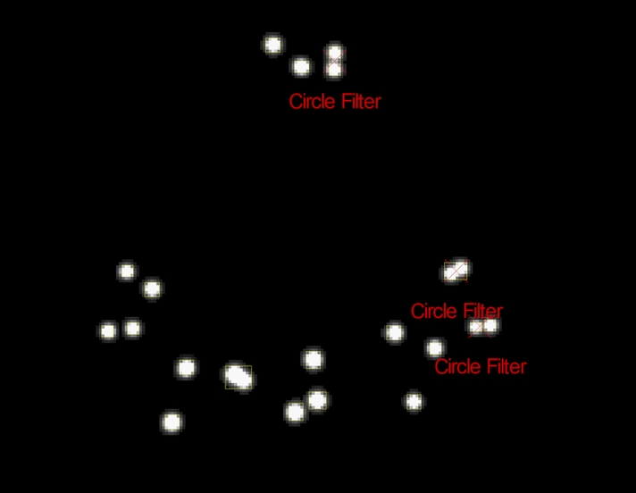
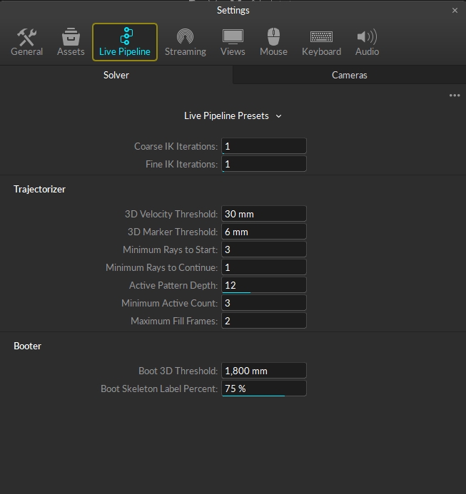
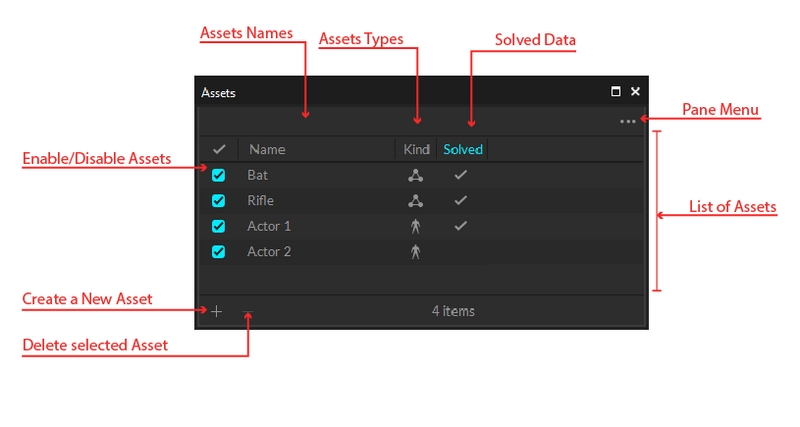
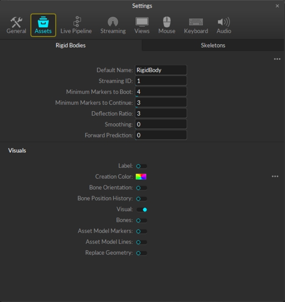
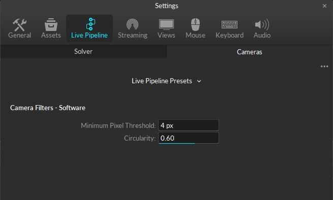
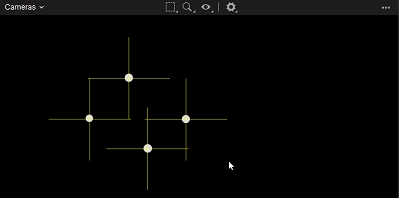
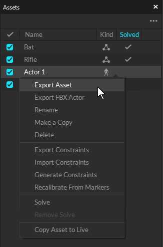
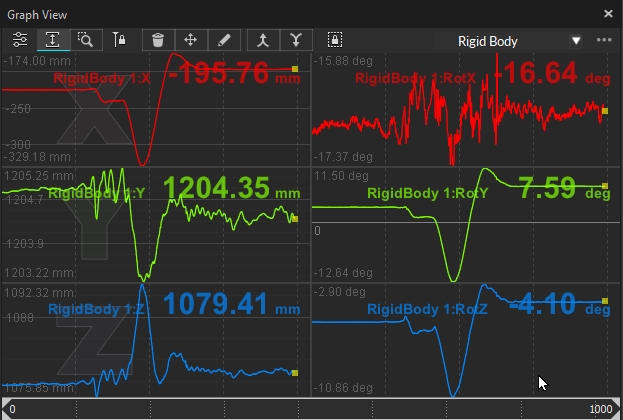
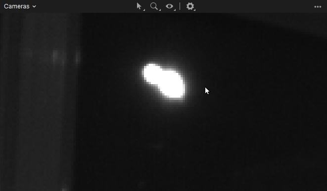
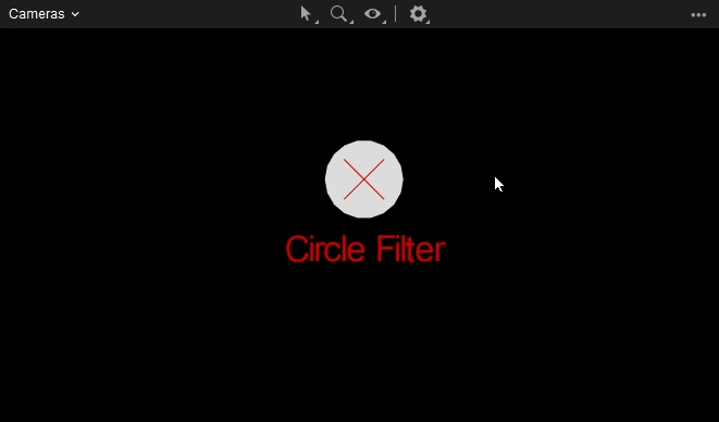
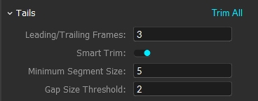
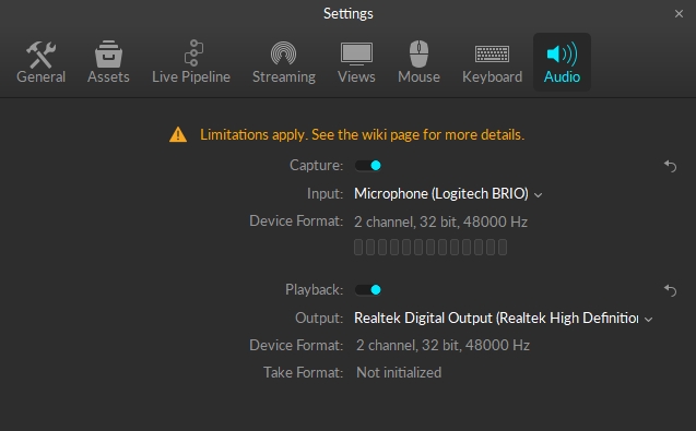
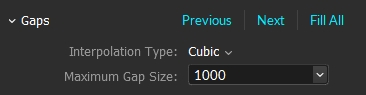
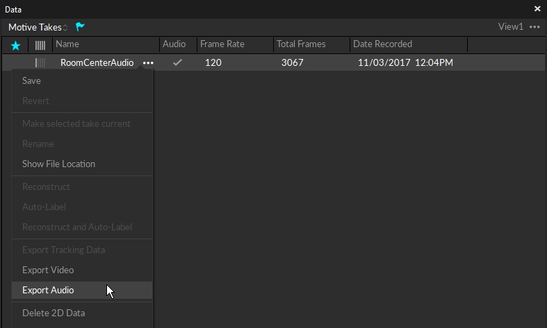
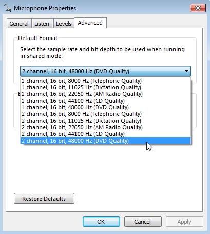
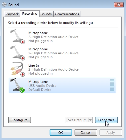
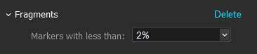
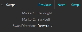
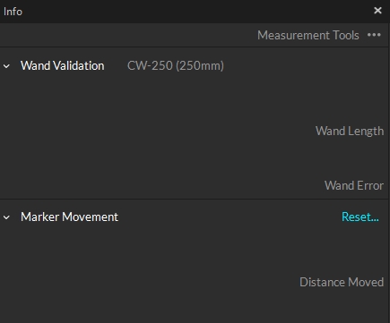
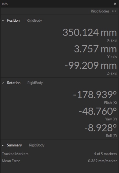
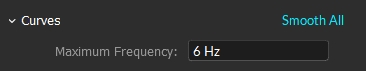
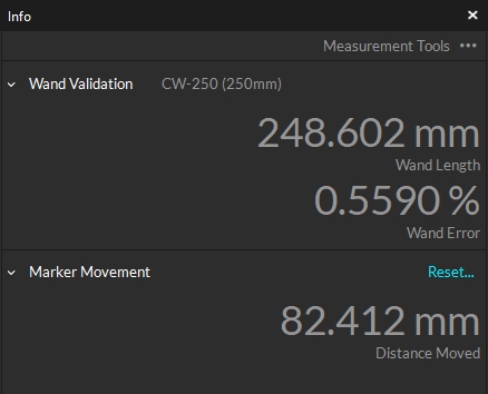
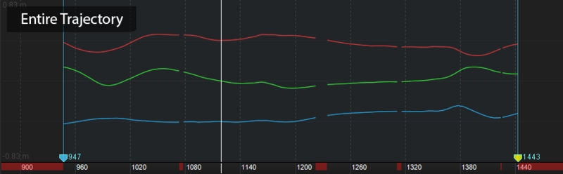

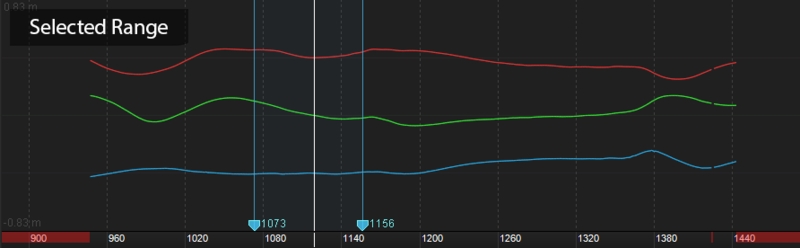

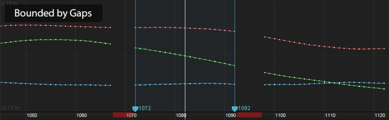
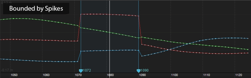


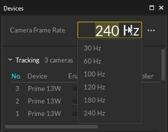

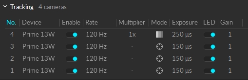
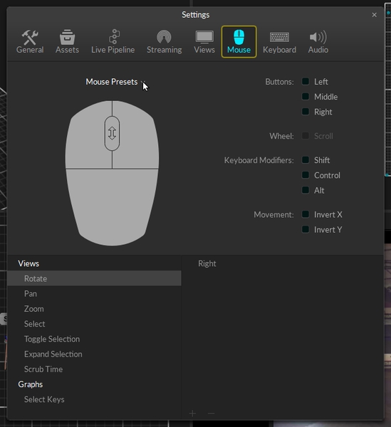
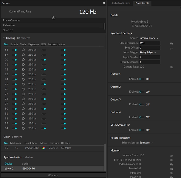
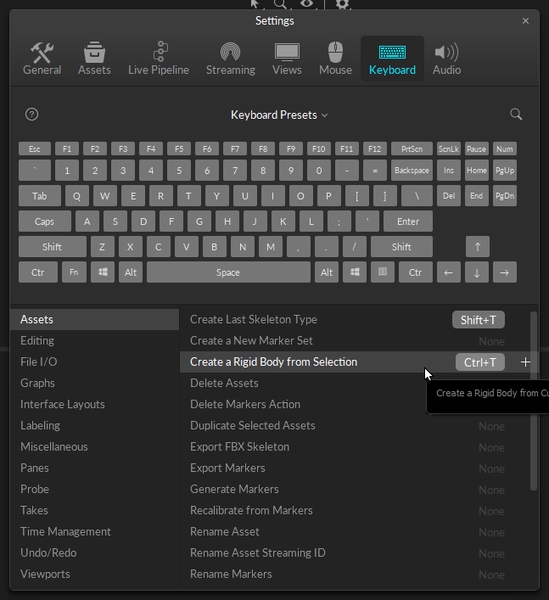
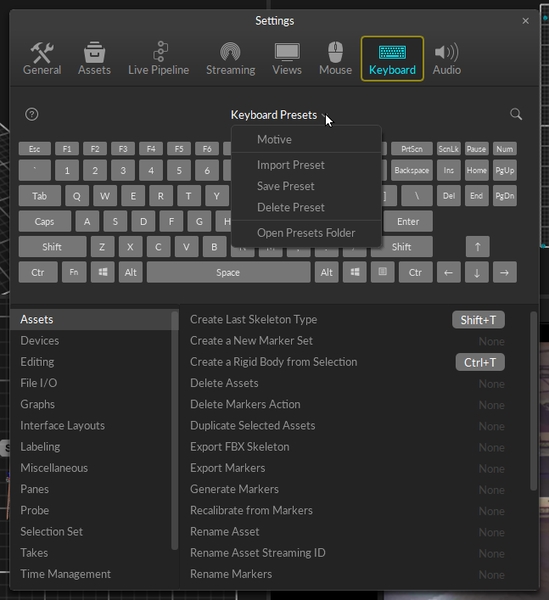
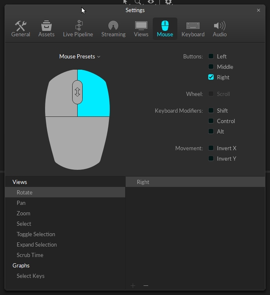
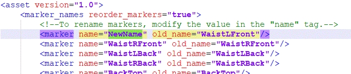
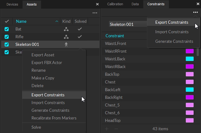
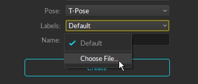
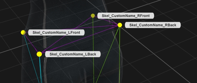
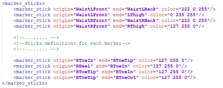
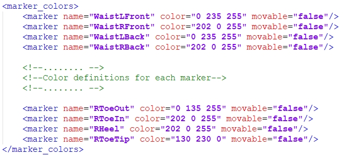
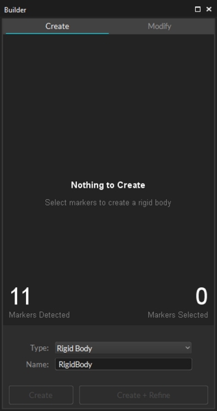
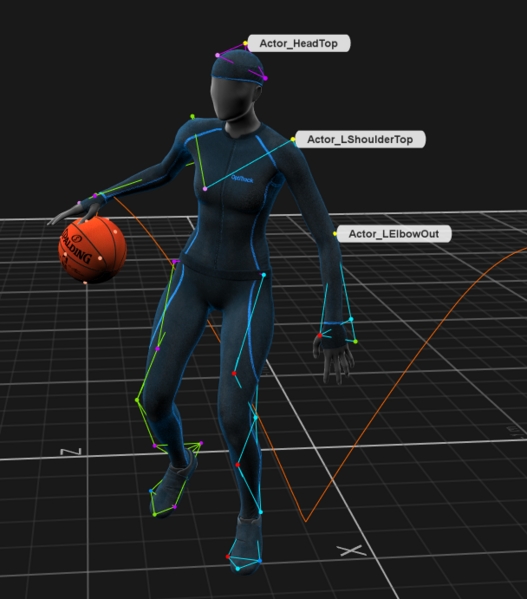
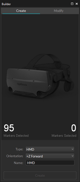
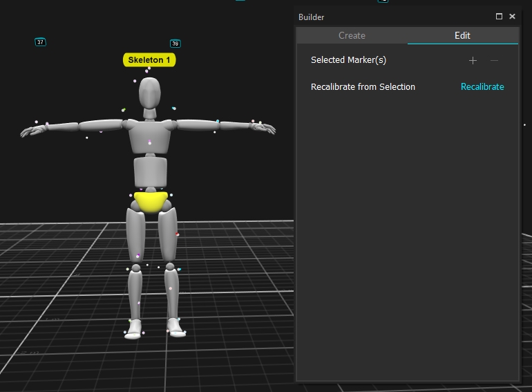
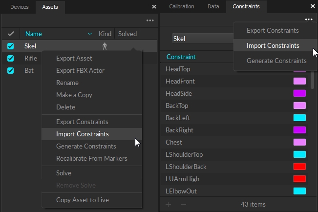
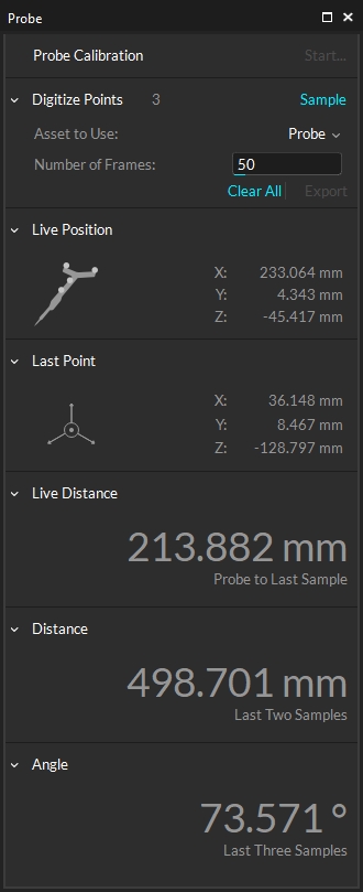
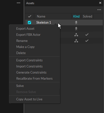
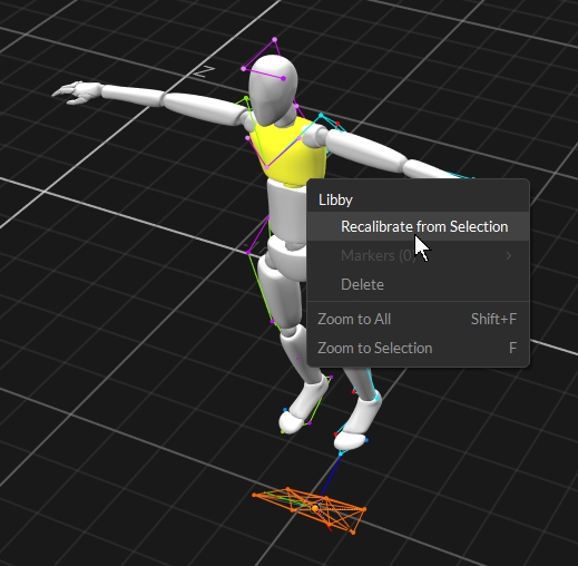
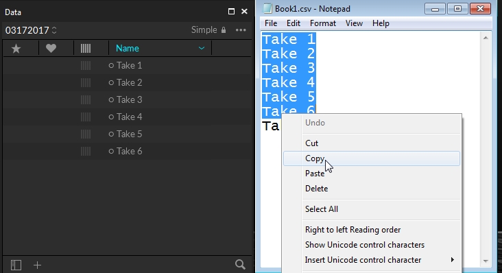
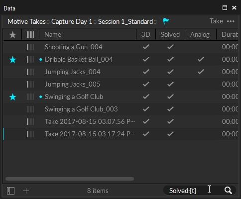
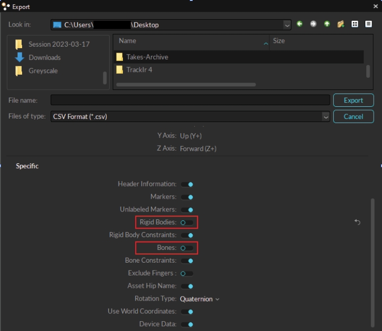
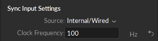
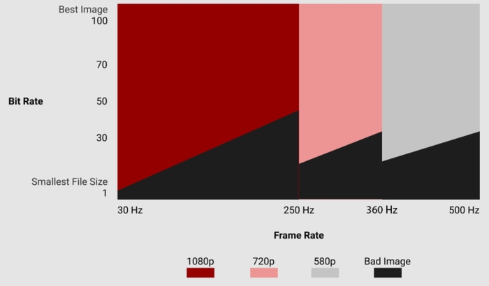
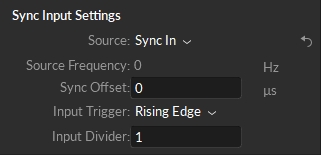
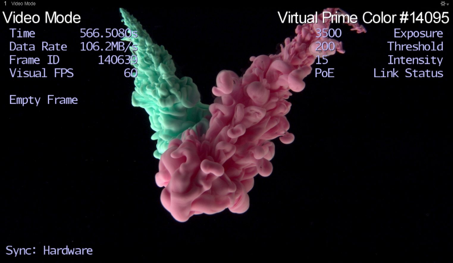
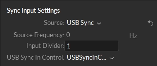
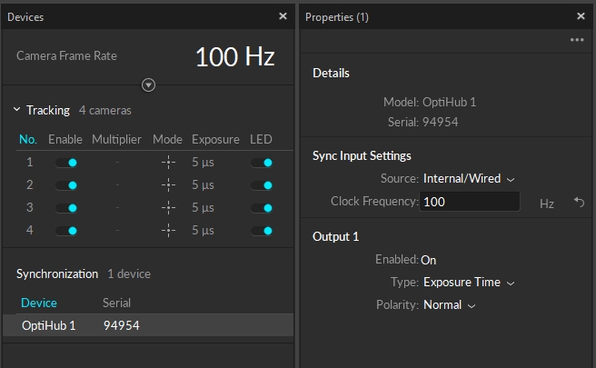
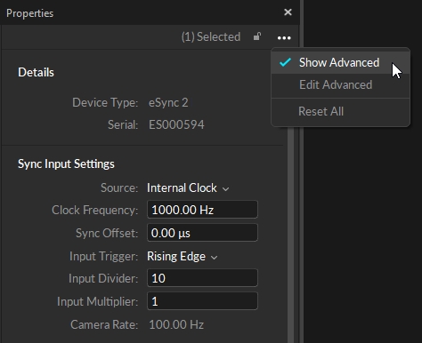
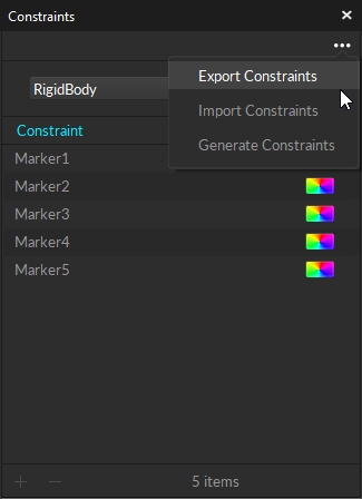
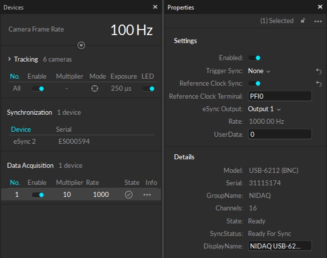


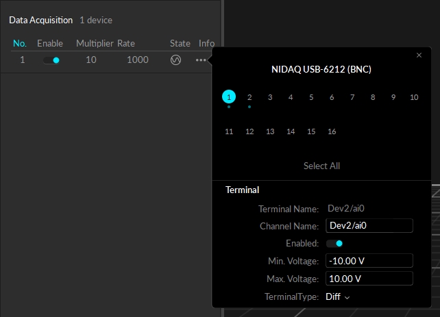
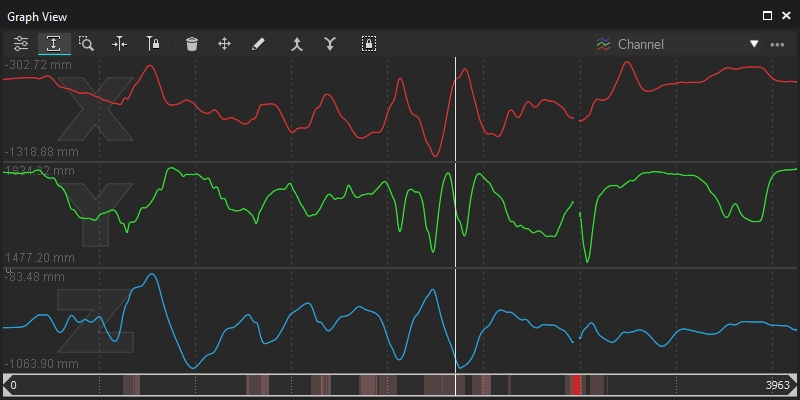
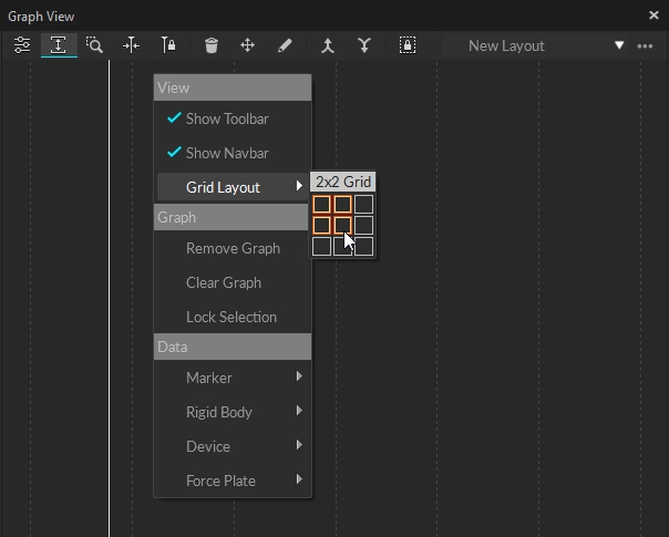
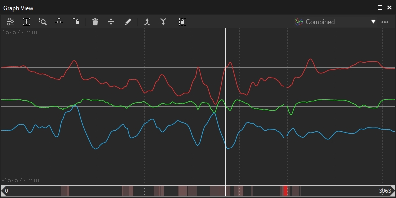
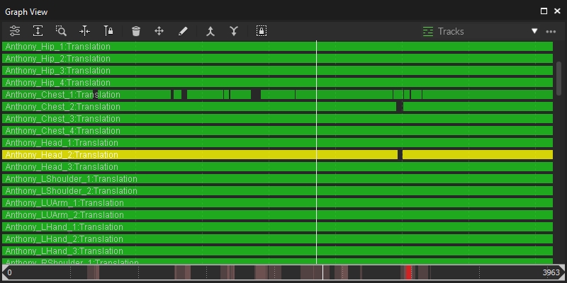
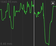
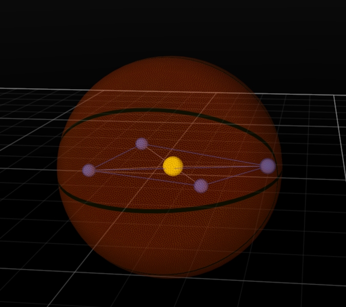
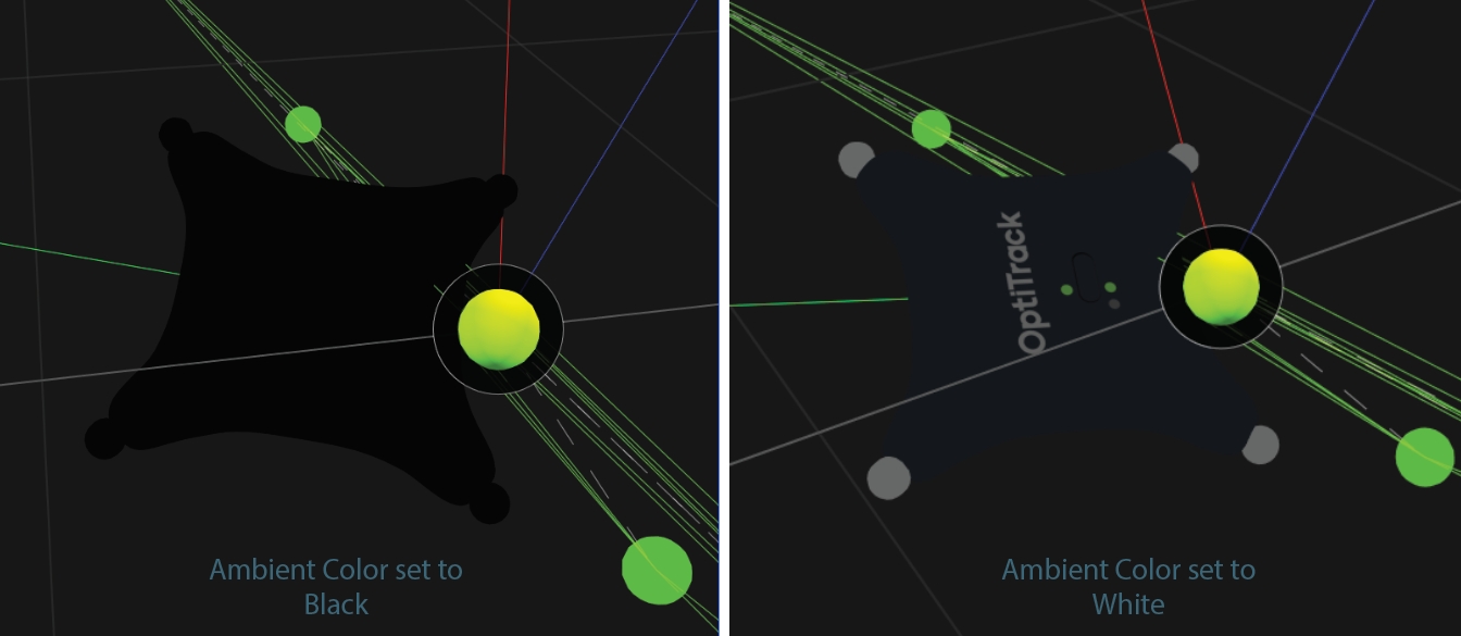
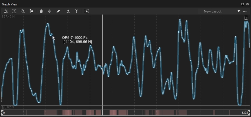


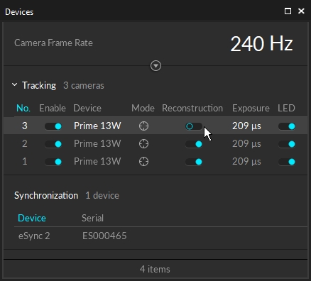
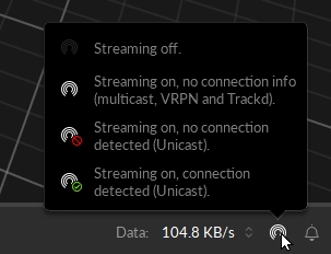
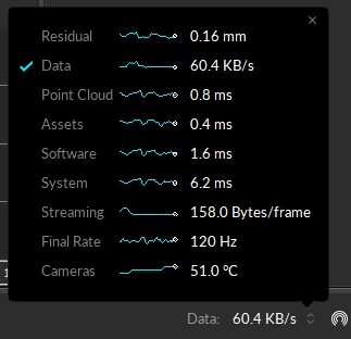
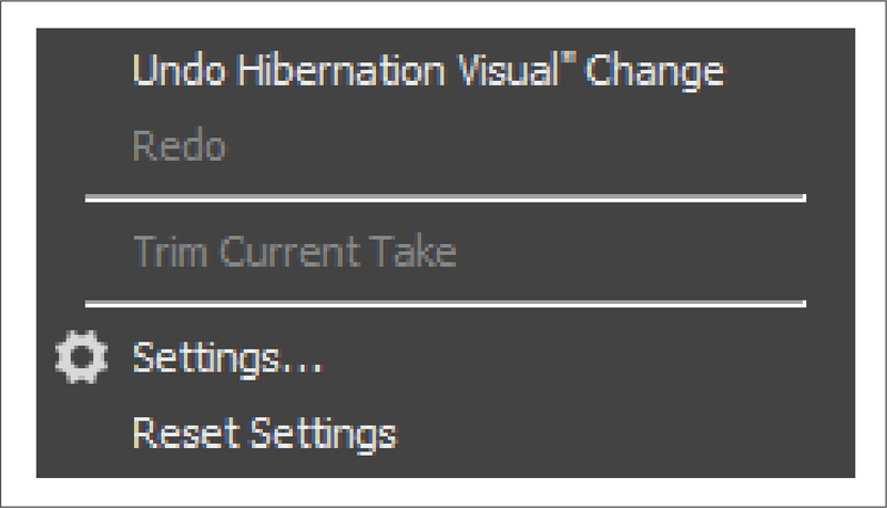
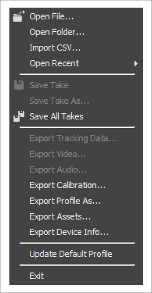
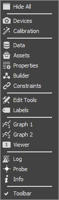
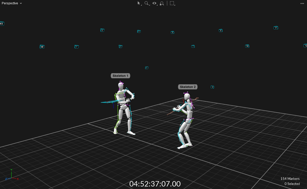
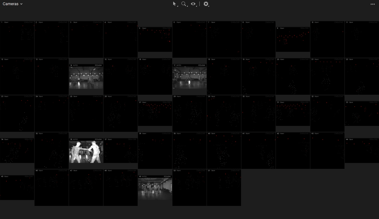
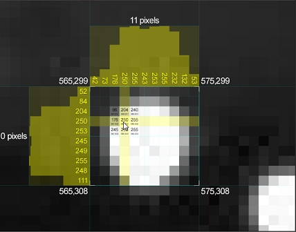
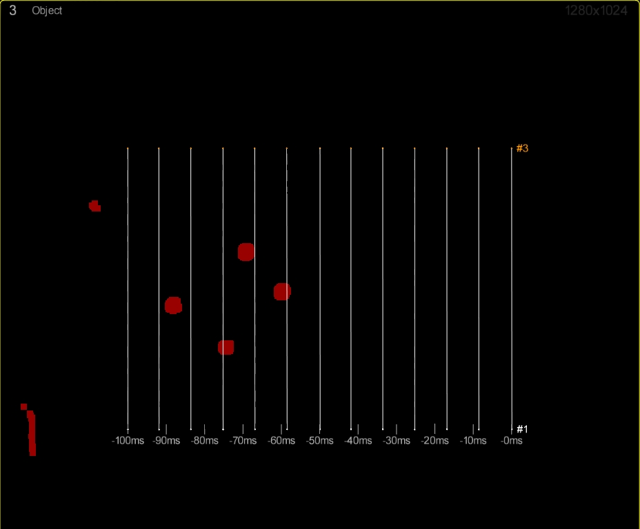
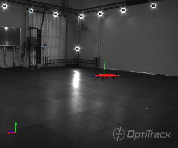
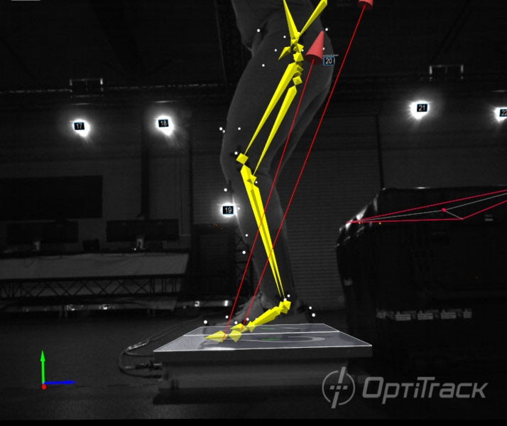
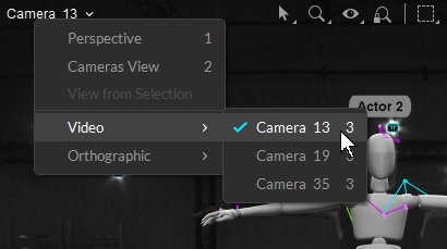
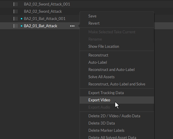
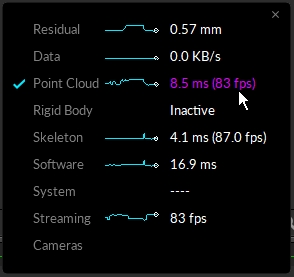